3 Concept of animation within the simulator
Imports
import os
os.chdir("../demo")
from pathlib import Path
from IPython.display import Code
from scripts.nb_utils import read_pc, read_from_output_folder, display_xml, download_from_url
import pyhelios
from pyhelios.util.xmldisplayer import find_playback_dir
import numpy as np
import pyvista as pv
pv.set_jupyter_backend('trame')
# url for getting the data
url = 'https://heibox.uni-heidelberg.de/f/2b264f8b55a94b749d51/?dl=1'
target_path = 'data/sceneparts'
Example 3.1: Tree moving in the wind during a single terrestrial laser scan
In terrestrial laser scanning (TLS) acquisitions, vegetation can appear as distorted if it is moving during the scan. These effects can be reproduced in the simulation. While vegetation actually deforms non-rigidly, we can assume that a single branch moves almost rigidly. We will therefore use a HELIOS++ dynamic scene with rigid motions to recreate the distortion effects. We create two dynamic scenes. In both cases, the branch rotates about its base, creating a way motion, but in opposite directions. With the scanner always rotating counter-clockwise, this will lead to a compressed branch (where scanner head and branch move in opposite directions) and an elongated branch (where scanner head and branch move in the same direction).
Getting the data
We first need to download the scene parts that we need for this example. Execute the code below!
download_from_url(url, target_path, subdir_path='Example_3-1')
Successfully downloaded and unpacked data to "data/sceneparts"
The scene
Dynamic scenes in HELIOS++ are defined in the XML files using motions (e.g., rotation and translation), which can be combined into one dmotion and chained together to motion sequences. We display just the first part of the scene XML below.
Code(display_xml('data/scenes/branch_anim_1.xml', line_limit=34), language='XML')
<document>
    <scene id="dyn_scene" name="Dynamic scene" dynTimeStep="0.020833333333333332">
        <part>
            <filter type="objloader">
                <param type="string" key="filepath" value="data/sceneparts/box/box_unit_test.obj" />
                <param type="string" key="up" value="z" />
            </filter>
            <filter type="scale">
                <param type="double" key="scale" value="0.15" />
            </filter>
        </part>
        <!--Dynamic scenepart-->
        <part>
            <filter type="objloader">
                <param type="string" key="filepath" value="data\sceneparts\animated_branch_1\leaves.obj" />
                <param type="string" key="up" value="z" />
            </filter>


            <dmotion id="leaves_0" loop="1" next="leaves_1">
              <motion type="rotation" axis="0.000;1.000;0.000" angle="0.00000000" center="0.00000000;0.00000000;0.00000000" autoCRS="1" />
              <motion type="translation" vec="0.00000000;0.00000000;0.00000000" />
            </dmotion>

            <dmotion id="leaves_1" loop="1" next="leaves_2">
              <motion type="rotation" axis="0.000;1.000;0.000" angle="0.00000000" center="0.00000000;0.00000000;0.00000000" autoCRS="1" />
              <motion type="translation" vec="0.00000000;0.00000000;0.00000000" />
            </dmotion>

            <dmotion id="leaves_2" loop="1" next="leaves_3">
              <motion type="rotation" axis="0.000;1.000;0.000" angle="0.00000000" center="0.00000000;0.00000000;0.00000000" autoCRS="1" />
              <motion type="translation" vec="0.00000000;0.00000000;0.00000000" />
            </dmotion>
Such a scene is of course difficult to write from scratch. We created this scene using the dyn_b2h Blender add-on for exporting Blender animations to HELIOS++ scenes. The add-on supports translations and rotations. Before starting the export, the animation should be baked to keyframes.
Let's have a quick look again what the static base scene looks like in 3D:
filepaths = Path('data/sceneparts/animated_branch_1').glob('*.obj')
p = pv.Plotter(notebook=True)
for f in filepaths:
    mesh = pv.read(f)
    p.add_mesh(mesh)
p.camera_position = 'yz'
p.show()
It's leaning to the right, and during the simulation, it will rotate around its bottom until it is leaning to the left.
The survey
The branch is simply scanned from a single position with a model of the RIEGL VZ-600i, which - as it supports a super high pulse frequency of 2,2 MHz - rotates pretty fast.
Code(display_xml('data/surveys/branch_anim_1.xml'), language='XML')
<document>
        <scannerSettings id="tls" active="true" pulseFreq_hz="2200000" verticalResolution_deg="0.017" horizontalResolution_deg="0.017" />
        <survey name="branch_anim_1" platform="data/platforms.xml#tripod" scanner="data/scanners_tls_custom.xml#riegl_vz600i" scene="data/scenes/branch_anim_1.xml#dyn_scene">
        <leg>
            <platformSettings x="-5" y="0" z="0" />
            <scannerSettings template="tls" headRotateStart_deg="260" headRotateStop_deg="280" trajectoryTimeInterval_s="0.05" />
        </leg>

        </survey>
    </document>
Executing the simulation
!helios data/surveys/branch_anim_1.xml -q --lasOutput --zipOutput --rebuildScene
output_path = Path(find_playback_dir('data/surveys/branch_anim_1.xml'))
pc_4d_1, object_id_1, _, _, gps_time_1, _ = read_from_output_folder(output_path)
idx = object_id_1 != 0
pc_4d_1 = pc_4d_1[idx, :]
gps_time_1 = gps_time_1[idx]
!helios data/surveys/branch_anim_2.xml -q --lasOutput --zipOutput --rebuildScene
output_path = Path(find_playback_dir('data/surveys/branch_anim_2.xml'))
pc_4d_2, object_id_2, _, _, gps_time_2, _ = read_from_output_folder(output_path)
idx = object_id_2 != 0
pc_4d_2 = pc_4d_2[idx, :]
gps_time_2 = gps_time_2[idx]
Visualizing the output
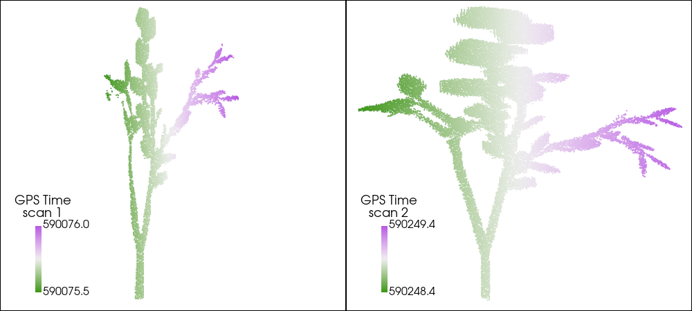
For the first scan, we expect the resulting point cloud to appear compressed in the y-direction as the branch moves in the opposite direction to the scanner. For the second scan, we expect that the branch to appear stretched, as it moves in the same direction as the scanner. Let's have a look.
sargs = {'title': 'GPS Time\nscan 1',
         'fmt': '%.1f',
         'n_labels': 2,
         'position_x': 0.1,
         'position_y': 0.05,
         'vertical': True,
         'height': 0.3,
         'width': 0.05,
         'label_font_size': 16}
p = pv.Plotter(notebook=True, shape=(1, 2), window_size=(1000, 450))
p.add_points(pc_4d_1,
             scalars=gps_time_1,
             style='points',
             cmap='gwv',
             point_size=2,
             scalar_bar_args=sargs)
p.subplot(0, 1)
sargs['title'] = 'GPS Time\nscan 2'
p.add_points(pc_4d_2,
             scalars=gps_time_2,
             style='points',
             cmap='gwv',
             point_size=2,
             scalar_bar_args=sargs)
p.link_views()
p.camera_position = 'yz'
p.camera.zoom(1.5)
p.show()