Multi-dimensional arrays: xarray¶

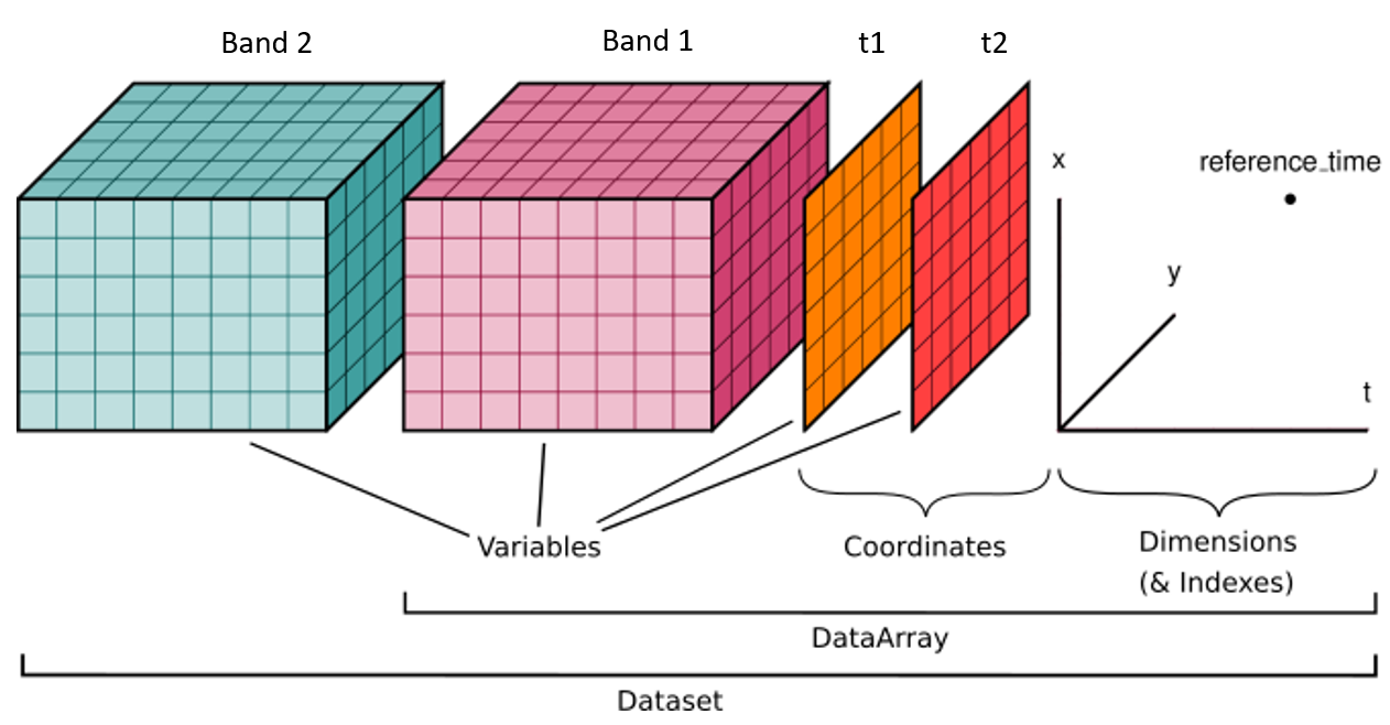
This short tutorial provides an introduction to raster handling with Python using the xarray package (Hoyer and Hamman 2017) for multi-dimensional data. Xarray's data structures (DataArray and Dataset, see here) complement NumPy-like arrays by labels in the form of dimensions, coordinates and attributes, thereby encoding information about how the array values are absolutely related to space, time etc. The labels can also be used to access and analyse the array values. These properties and functionality are very useful if you work with time series of remote sensing images or other raster data. Many of the visualizations in this tutorial could be improved with a few lines of code (e.g. to add axes labels and plot titles) or by using specialized plotting packages, but here we try to keep the code simple.

Xarray Dataset structure. Spectral bands can be treated as data variables, time as a dimension in addition to the spatial dimensions (modified from the xarray User Guide).

Data

As a sample dataset, we use a a single GeoTiff file with six bands. This imagery was acquired by one of the two Sentinel-2 satellites and covers a relatively small area around the village of Obergurgl, located in the Central Alps of Tyrol (Austria). This imagery has been queried from the Google Earth Engine (GEE), then cloud-masked and exported from GEE.

Getting started with xarray's data structures and basic tools¶

Loading and handling single images¶

In this tutorial, we start with importing and exploring an individual image. So we load a single GeoTiff file with six bands. A good way to do this is using rioxarray, a geospatial xarray extension powered by rasterio. Rioxarray extends xarray by improved support for geospatial metadata, as rasterio does for numpy arrays.

In [1]:

import rioxarray
import xarray
from pathlib import Path

import rioxarray import xarray from pathlib import Path

In [2]:

# Open a GeoTiff from a local directory using the rio accessor
data_dir = Path('F:/data/etrainee/gee')        # Define the path to the s2 directory with the Sentinel-2 image subsets on your local system
in_file = data_dir / 's2' / '20180726T102019_20180726T102150_T32TPS.tif' # Specify the path and the filename of an image
xds = rioxarray.open_rasterio(in_file, masked=True)     # Read the mask (NoData in the GeoTiff) and set values to NaN (for proper interpretation by xarray)

# Open a GeoTiff from a local directory using the rio accessor data_dir = Path('F:/data/etrainee/gee') # Define the path to the s2 directory with the Sentinel-2 image subsets on your local system in_file = data_dir / 's2' / '20180726T102019_20180726T102150_T32TPS.tif' # Specify the path and the filename of an image xds = rioxarray.open_rasterio(in_file, masked=True) # Read the mask (NoData in the GeoTiff) and set values to NaN (for proper interpretation by xarray)

Print some information about the xarray.DataArray called 'xds':

In [6]:

xds

xds

Out[6]:

<xarray.DataArray (band: 6, y: 201, x: 251)>
[302706 values with dtype=float32]
Coordinates:
  * band         (band) int32 1 2 3 4 5 6
  * x            (x) float64 6.516e+05 6.516e+05 ... 6.566e+05 6.566e+05
  * y            (y) float64 5.194e+06 5.194e+06 5.194e+06 ... 5.19e+06 5.19e+06
    spatial_ref  int32 0
Attributes:
    AREA_OR_POINT:           Area
    TIFFTAG_RESOLUTIONUNIT:  1 (unitless)
    TIFFTAG_XRESOLUTION:     1
    TIFFTAG_YRESOLUTION:     1
    scale_factor:            1.0
    add_offset:              0.0

xarray.DataArray

• band: 6
• y: 201
• x: 251

• ...

  [302706 values with dtype=float32]

• Coordinates: (4)
  • band
    (band)
    int32
    1 2 3 4 5 6

    array([1, 2, 3, 4, 5, 6])

  • x
    (x)
    float64
    6.516e+05 6.516e+05 ... 6.566e+05

    array([651590., 651610., 651630., ..., 656550., 656570., 656590.])

  • y
    (y)
    float64
    5.194e+06 5.194e+06 ... 5.19e+06

    array([5193750., 5193730., 5193710., ..., 5189790., 5189770., 5189750.])

  • spatial_ref
    ()
    int32
    0

    crs_wkt :

    PROJCS["WGS 84 / UTM zone 32N",GEOGCS["WGS 84",DATUM["WGS_1984",SPHEROID["WGS 84",6378137,298.257223563,AUTHORITY["EPSG","7030"]],AUTHORITY["EPSG","6326"]],PRIMEM["Greenwich",0,AUTHORITY["EPSG","8901"]],UNIT["degree",0.0174532925199433,AUTHORITY["EPSG","9122"]],AUTHORITY["EPSG","4326"]],PROJECTION["Transverse_Mercator"],PARAMETER["latitude_of_origin",0],PARAMETER["central_meridian",9],PARAMETER["scale_factor",0.9996],PARAMETER["false_easting",500000],PARAMETER["false_northing",0],UNIT["metre",1,AUTHORITY["EPSG","9001"]],AXIS["Easting",EAST],AXIS["Northing",NORTH],AUTHORITY["EPSG","32632"]]

    semi_major_axis :

    6378137.0

    semi_minor_axis :

    6356752.314245179

    inverse_flattening :

    298.257223563

    reference_ellipsoid_name :

    WGS 84

    longitude_of_prime_meridian :

    0.0

    prime_meridian_name :

    Greenwich

    geographic_crs_name :

    WGS 84

    horizontal_datum_name :

    World Geodetic System 1984

    projected_crs_name :

    WGS 84 / UTM zone 32N

    grid_mapping_name :

    transverse_mercator

    latitude_of_projection_origin :

    0.0

    longitude_of_central_meridian :

    9.0

    false_easting :

    500000.0

    false_northing :

    0.0

    scale_factor_at_central_meridian :

    0.9996

    spatial_ref :

    PROJCS["WGS 84 / UTM zone 32N",GEOGCS["WGS 84",DATUM["WGS_1984",SPHEROID["WGS 84",6378137,298.257223563,AUTHORITY["EPSG","7030"]],AUTHORITY["EPSG","6326"]],PRIMEM["Greenwich",0,AUTHORITY["EPSG","8901"]],UNIT["degree",0.0174532925199433,AUTHORITY["EPSG","9122"]],AUTHORITY["EPSG","4326"]],PROJECTION["Transverse_Mercator"],PARAMETER["latitude_of_origin",0],PARAMETER["central_meridian",9],PARAMETER["scale_factor",0.9996],PARAMETER["false_easting",500000],PARAMETER["false_northing",0],UNIT["metre",1,AUTHORITY["EPSG","9001"]],AXIS["Easting",EAST],AXIS["Northing",NORTH],AUTHORITY["EPSG","32632"]]

    GeoTransform :

    651580.0 20.0 0.0 5193760.0 0.0 -20.0

    array(0)

• Indexes: (3)
  • band
    PandasIndex

    PandasIndex(Index([1, 2, 3, 4, 5, 6], dtype='int32', name='band'))

  • x
    PandasIndex

    PandasIndex(Index([651590.0, 651610.0, 651630.0, 651650.0, 651670.0, 651690.0, 651710.0,
           651730.0, 651750.0, 651770.0,
           ...
           656410.0, 656430.0, 656450.0, 656470.0, 656490.0, 656510.0, 656530.0,
           656550.0, 656570.0, 656590.0],
          dtype='float64', name='x', length=251))

  • y
    PandasIndex

    PandasIndex(Index([5193750.0, 5193730.0, 5193710.0, 5193690.0, 5193670.0, 5193650.0,
           5193630.0, 5193610.0, 5193590.0, 5193570.0,
           ...
           5189930.0, 5189910.0, 5189890.0, 5189870.0, 5189850.0, 5189830.0,
           5189810.0, 5189790.0, 5189770.0, 5189750.0],
          dtype='float64', name='y', length=201))

• Attributes: (6)

  AREA_OR_POINT :

  Area

  TIFFTAG_RESOLUTIONUNIT :

  1 (unitless)

  TIFFTAG_XRESOLUTION :

  1

  TIFFTAG_YRESOLUTION :

  1

  scale_factor :

  1.0

  add_offset :

  0.0

Or more specifically:

In [7]:

print(xds.shape)
print(xds.dims)
print(xds.coords)

print(xds.shape) print(xds.dims) print(xds.coords)

(6, 201, 251)
('band', 'y', 'x')
Coordinates:
  * band         (band) int32 1 2 3 4 5 6
  * x            (x) float64 6.516e+05 6.516e+05 ... 6.566e+05 6.566e+05
  * y            (y) float64 5.194e+06 5.194e+06 5.194e+06 ... 5.19e+06 5.19e+06
    spatial_ref  int32 0

... and some descriptive statistics for one band (using xarray's built-in methods, but numpy could be used as well):

In [8]:

# Extract a band to a new DataArray (for conveniance)
band_1 =xds.sel(band=1)
print('min: ', band_1.min().values)     # Print only the value(s) of the array; its only one value for one band and one time stamp 
print('max: ', band_1.max().values)
print('mean: ', band_1.mean().values)
print('std: ', band_1.std().values)

# Extract a band to a new DataArray (for conveniance) band_1 =xds.sel(band=1) print('min: ', band_1.min().values) # Print only the value(s) of the array; its only one value for one band and one time stamp print('max: ', band_1.max().values) print('mean: ', band_1.mean().values) print('std: ', band_1.std().values)

min:  138.0
max:  6651.0
mean:  666.3916
std:  358.31906

We can use the extended capabilities of rioxarray to query more metadata, such as coordinate reference system (CRS), bounding coordinates, dimensions, spatial resolution, or defined NoData value:

In [9]:

print(xds.rio.crs)
print(xds.rio.bounds())
print(xds.rio.width)
print(xds.rio.height)
print(xds.rio.resolution())
print(xds.rio.nodata)

print(xds.rio.crs) print(xds.rio.bounds()) print(xds.rio.width) print(xds.rio.height) print(xds.rio.resolution()) print(xds.rio.nodata)

EPSG:32632
(651580.0, 5189740.0, 656600.0, 5193760.0)
251
201
(20.0, -20.0)
nan

Plotting DataArrays¶

Creating a new DataArray with only one selected band is straightforward and plotting this is easy as well (matplotlib must be installed in the active conda environment). Note the white NoData areas due to cloud masking:

In [10]:

band_1 = xds.sel(band=1)            # Select a band by its label (or by its index with '.isel()'), as already shown above
band_1.plot.imshow(robust=True)     # The 'robust' option stretches the colormap range to 2nd and 98th percentiles.

band_1 = xds.sel(band=1) # Select a band by its label (or by its index with '.isel()'), as already shown above band_1.plot.imshow(robust=True) # The 'robust' option stretches the colormap range to 2nd and 98th percentiles.

Out[10]:

<matplotlib.image.AxesImage at 0x28681981960>

Now let's create a histogram for this band. We use xarray.plot.hist(), for more advanced options there are the xhistogram and the boost-histogram packages. You might try different estimators to determine the optimum number of bins (see here; default would be 10 bins; 'auto' takes the maximum of the Sturges and Freedman Diaconis estimators).

In [11]:

xds.sel(band=1).plot.hist(bins='auto'); # The semicolon tells Jupyter Notebook not to display the output of that line of code (i.e. the bin values; but it will show the histogram).

xds.sel(band=1).plot.hist(bins='auto'); # The semicolon tells Jupyter Notebook not to display the output of that line of code (i.e. the bin values; but it will show the histogram).

Similarly, we can plot 3-band combinations as true-color or false-color (color-infrared, CIR) image by selecting the bands to plot as RGB:

In [12]:

xds.sel(band=[3, 2, 1]).plot.imshow(robust=True)

xds.sel(band=[3, 2, 1]).plot.imshow(robust=True)

Out[12]:

<matplotlib.image.AxesImage at 0x28682744100>

c:\Users\Andi\mambaforge\envs\geopython\lib\site-packages\matplotlib\cm.py:494: RuntimeWarning: invalid value encountered in cast
  xx = (xx * 255).astype(np.uint8)

In [13]:

xds.sel(band=[4, 3, 2]).plot.imshow(robust=True)

xds.sel(band=[4, 3, 2]).plot.imshow(robust=True)

Out[13]:

<matplotlib.image.AxesImage at 0x286827ca470>

Instead of using robust=True we could also constrain the color stretch to the respective quantiles using the vmin and vmax keyword arguments. Try also other quantiles or explicit values and see how this affects the image display.

In [14]:

xds.sel(band=[3, 2, 1]).plot.imshow(
    vmin=xds.sel(band=[3, 2, 1]).quantile(0.02),
    vmax=xds.sel(band=[3, 2, 1]).quantile(0.98))

xds.sel(band=[3, 2, 1]).plot.imshow( vmin=xds.sel(band=[3, 2, 1]).quantile(0.02), vmax=xds.sel(band=[3, 2, 1]).quantile(0.98))

Out[14]:

<matplotlib.image.AxesImage at 0x28682618ac0>

c:\Users\Andi\mambaforge\envs\geopython\lib\site-packages\matplotlib\cm.py:494: RuntimeWarning: invalid value encountered in cast
  xx = (xx * 255).astype(np.uint8)

Now you know how to work with xarray on a single multispectral image and you are ready to expand this by the time dimension. Several tutorials of E-TRAINEE Module 1 use xarray to handle satellite image time series.