Basic bi-temporal change analysis
This tutorial demonstrates the standard workflow for performing a bi-temporal change analysis using the M3C2 algorithm (Lague et al., 2013) implemented in py4dgeo. It covers the entire process from importing point cloud data, running the M3C2 algorithm, to visualizing the resulting M3C2 distances.
Learning Objectives:
- Understand the M3C2 algorithm for 3D point cloud comparison.
- Load point cloud epochs using
py4dgeo. - Configure and run the M3C2 algorithm.
- Visualize and interpret the resulting change distances.
- Save the M3C2 results to a LAS file.
- Learn how to customize the algorithm.
Dataset
As example data, we are using a time series of TLS-based snow cover monitoring acquired at the Zugspitze, Germany (see visualization below). The data are openly available on the PANGAEA data repository (Anders et al., 2022). Here, we provide a subset of the data to reduce the volume. The data covers a smaller area of interest in the scene, namely part of the snow-covered slope, and is subsampled to a point spacing of 50 cm. The hourly point clouds cover 107 epochs acquired in April 2019. This dataset will be used for all tutorials in Activity 2.
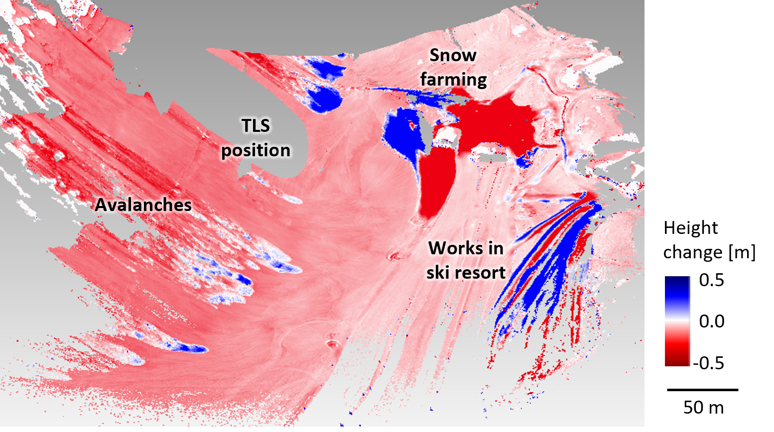
Bitemporal point cloud distances of snow-covered scene acquired by terrestrial laser scanning (TLS) within a three-day timespan, where avalanche erosion and deposition forms overlap with overall decrease of the snow cover. Figure by K. Anders, following Anders et al. (2022).
What is M3C2?
The M3C2 (Multiscale Model-to-Model Cloud Comparison) algorithm is a robust method for computing distances directly between two point clouds. Unlike simple cloud-to-cloud distance calculations, M3C2 has two key advantages:
- Local Surface Normals: It calculates distances along the direction of the local surface normal at each point. This provides a more accurate and physically meaningful measure of change, especially on complex 3D surfaces.
- Multi-scale Analysis: It uses a spherical neighborhood to calculate the surface roughness. This allows it to distinguish between actual surface change and noise, providing a confidence value for each calculated distance.
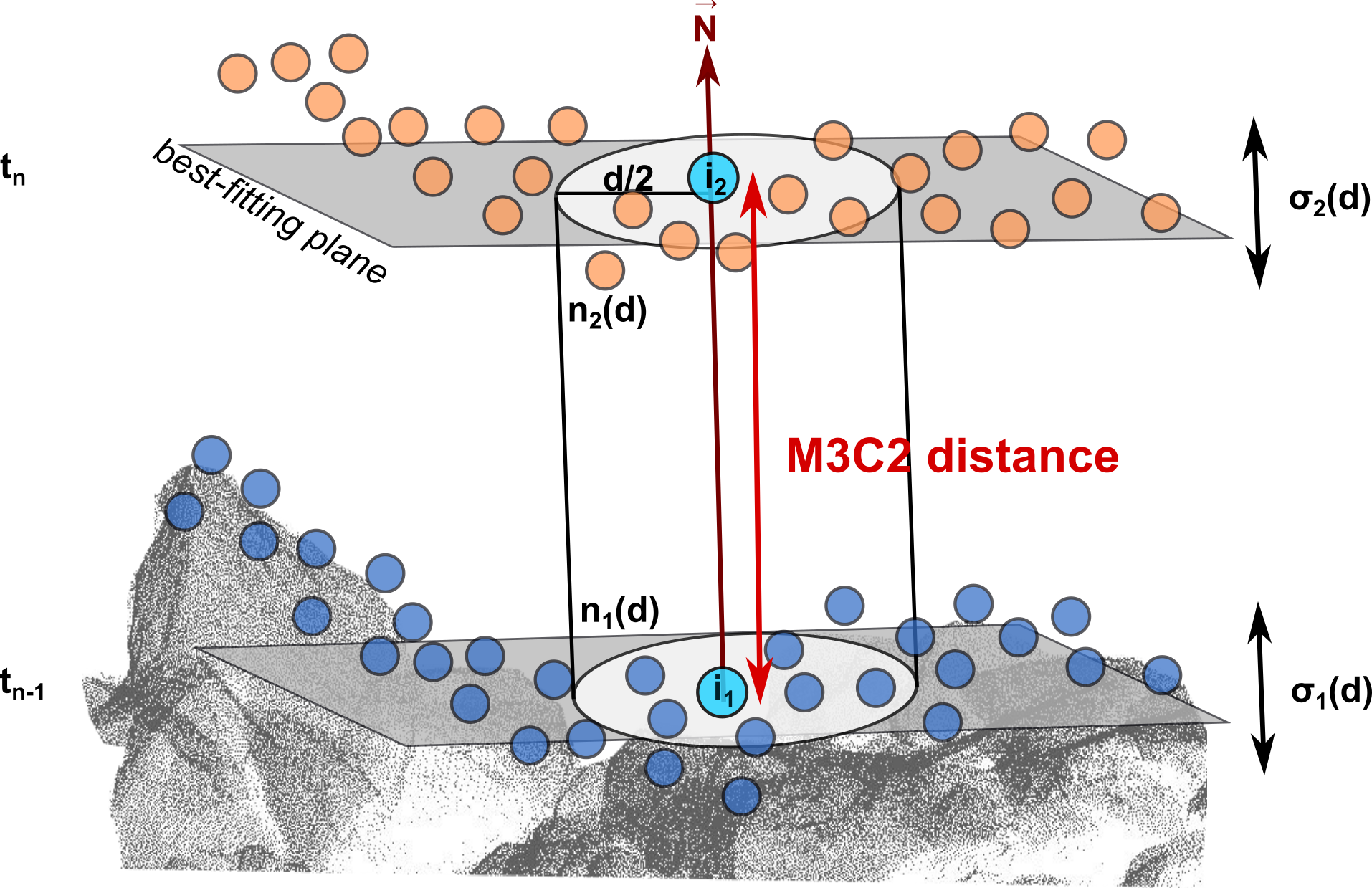
Schematic of point cloud distance computation with the M3C2 algorithm (Lague et al., 2013). Figure by V. Zahs modified from Zahs et al. (2022).
Setup and Data Loading
First, we import the necessary libraries. We'll need py4dgeo for the main computation and matplotlib for plotting our results.
from pathlib import Path
import py4dgeo
import numpy as np
import matplotlib.pyplot as plt
Now, we need to load two datasets that cover the same scene at two different points in time. Point cloud datasets are represented by numpy arrays of shape n x 3 using a 64 bit floating point type (np.float64). py4dgeo supports reading point clouds from both LAS/LAZ files using read_from_las and text-based XYZ files using read_from_xyz.
For this tutorial, we will use the following 2 epochs from the dataset.
# load the data
data_path = Path("../data/activity_2/point_clouds")

epoch1_path = data_path / "schneeferner_180419_150005.laz"
epoch2_path = data_path / "schneeferner_180419_160005.laz"

epoch1 = py4dgeo.read_from_las(epoch1_path)
epoch2 = py4dgeo.read_from_las(epoch2_path)

print(f"Loaded epoch 1 with {epoch1.cloud.shape[0]} points.")
print(f"Loaded epoch 2 with {epoch2.cloud.shape[0]} points.")
Let's visualize the first epoch to get an idea of the scene we are working with.
fig = plt.figure(figsize=(8, 6))
ax = fig.add_subplot(projection='3d')
nth=10
ax.scatter(epoch1.cloud[::nth, 0], epoch1.cloud[::nth, 1], epoch1.cloud[::nth, 2], s=1, c=epoch1.cloud[::nth, 2])
ax.set_xlabel("X")
ax.set_ylabel("Y")
ax.set_zlabel("Z")
ax.set_title("Epoch 1 Point Cloud (subsampled for visualization)")
ax.view_init(elev=30, azim=120)
plt.show()

M3C2 distances
The analysis of point cloud distances is executed on so-called core points (Lague et al., 2013). These could be, e.g., one of the input point clouds, a subsampled version thereof, points in an equidistant grid, etc. Here, we choose a subsampling by taking every second point of the reference point cloud:
corepoints = epoch1.cloud[::2]
Now we are ready to set up and run the M3C2 algorithm. Let's take a closer look at the parameters we are using to instantiate the M3C2 class:
epochs=(epoch1, epoch2): This is a tuple containing the two point clouds (from different times) that we want to compare.epoch1is treated as the reference cloud, andepoch2as the target cloud.corepoints=corepoints: These are the specific points at which the M3C2 distances will be calculated. The algorithm will compute one distance value for each point in this array.cyl_radius=2.0: This is the projection cylinder radius. For each core point, M3C2 projects the local neighborhood of points from both clouds into a cylinder to calculate the average distance. This radius defines the size of the cylinder.normal_radii=[0.5, 1.0, 2.0]: This is a list of radii used for calculating the surface normal at each core point. This parameter enables the multi-scale nature of M3C2. The algorithm calculates a surface normal for each of the provided radii and then evaluates the "planarity" of the surface at each scale. It automatically selects the normal from the radius that corresponds to the flattest local surface (i.e., the most reliable scale for determining the surface orientation).- A small radius is good for capturing fine details on a complex surface.
- A large radius is better for smoothing over noise on a generally flat surface.
By providing a list of radii, you allow the algorithm to adaptively choose the most appropriate scale for each individual core point.
m3c2 = py4dgeo.M3C2(
    epochs=(epoch1, epoch2),
    corepoints=corepoints,
    cyl_radius=2.0,
    normal_radii=[0.5, 1.0, 2.0],
)

distances, uncertainties = m3c2.run()
[2026-06-23 14:49:22][INFO] Building KDTree structure with leaf parameter 10
[2026-06-23 14:49:22][INFO] Building KDTree structure with leaf parameter 10
The calculated result is an array with one distance per core point. The order of distances corresponds exactly to the order of input core points.
distances
array([-0.00658198, -0.01189156, -0.00646773, ...,  0.00523213,
        0.00089233,  0.0070209 ], shape=(74096,))
Visualization
Now that we have the distances, the best way to interpret them is to visualize them on the point cloud. We will create a 3D scatter plot of our core points, and use the M3C2 distances to color each point.
This will give us a clear spatial understanding of where changes have occurred. We will use a diverging colormap (coolwarm_r) where:
- Red indicates negative change (e.g., erosion, material loss).
- Blue indicates positive change (e.g., deposition, material gain).
- White indicates areas with little to no change.
We will also set a threshold (vmax) to cap the color scale, which helps to highlight subtle changes and prevent extreme outliers from dominating the visualization.
# Set a threshold for the color bar to make visualization clearer
vmax = 0.6
fig = plt.figure(figsize=(8, 6))
ax = fig.add_subplot(projection='3d')
sc = ax.scatter(
    corepoints[:, 0],
    corepoints[:, 1],
    corepoints[:, 2],
    c=distances,
    cmap='coolwarm_r',
    s=1,
    vmin=-vmax,
    vmax=vmax
)
cbar = plt.colorbar(sc, ax=ax, shrink=0.6, pad=0.12)
cbar.set_label('M3C2 Distance (m)')
ax.set_xlabel("X")
ax.set_ylabel("Y")
ax.set_zlabel("Z")
ax.set_title("M3C2 Distances on Core Points")
ax.set_aspect('equal', 'box')
ax.view_init(elev=30, azim=120)

plt.show()

Uncertainty metrics
Corresponding to the derived distances, an uncertainty array is returned which contains several quantities that can be accessed individually: The level of detection lodetection, the spread of the distance across points in either cloud (spread1 and spread2, by default measured as the standard deviation of distances) and the total number of points taken into consideration in either cloud (num_samples1 and num_samples2):"
uncertainties["lodetection"]
array([0.01131072, 0.01329877, 0.01950299, ..., 0.34346117, 0.31022056,
       0.32645114], shape=(74096,))
uncertainties["spread1"]
array([0.01215401, 0.01802715, 0.0361245 , ..., 0.71380526, 0.65211375,
       0.65714432], shape=(74096,))
uncertainties["num_samples1"]
array([14, 22, 28, ..., 33, 35, 32], shape=(74096,))
The direction of surface change in the M3C2 algorithm is determined via local normal vectors per core point. The normal vectors used in the calculation can be accessed via the directions() method of the M3C2 algorithm in py4dgeo, which returns an array (Nx3) of length N corresponding to the number of core points with three entries for the normal vector components in x, y, and z direction.
directions = m3c2.directions()
The property directions_radii returns an array (Nx1) of length N corresponding to the number of core points and one entry for the radius used for normal computation at the respective core point. This is relevant for the multi-scale functionality of the M3C2, i.e. the possibility to specify multiple normal radii of which the one with maximized planarity is used for change analysis.
direction_radii = m3c2.directions_radii()
Save output
After running the M3C2 algorithm, you can save the results as a LAS file. The write_m3c2_results_to_las function exports the corepoints along with their calculated attributes.
outputfilepath = "m3c2_results.las"
attributes_to_save = {
    "distance": distances,  # The M3C2 distances
    "lodetection": uncertainties["lodetection"],  # Level of detection
    "spread1": uncertainties["spread1"],  # Spread in first cloud
    "spread2": uncertainties["spread2"],  # Spread in second cloud
    "num_points1": uncertainties["num_samples1"],  # Number of points in first cloud
    "num_points2": uncertainties["num_samples2"],  # Number of points in second cloud
    "normal_x": directions[:, 0],  # X component of normal vector
    "normal_y": directions[:, 1],  # Y component of normal vector
    "normal_z": directions[:, 2],  # Z component of normal vector
    "normal_radius": direction_radii,  # Radius used for normal computation
}

py4dgeo.write_m3c2_results_to_las(outputfilepath, m3c2, attributes_to_save)
if Path(outputfilepath).exists():
    print(f"Results successfully saved to: {Path(outputfilepath).resolve()}")
else:
    print("Failed to save results.")
Algorithm customization
py4dgeo does not only provide a high performance implementation of the M3C2 base algorithm and some of it variants. It also allows you to rapidly prototype new algorithms in Python. We will demonstrate the necessary concepts by implementing some dummy algorithms without geographic relevance.
Inherting from the algorithm class
Each algorithm is represented by a class that inherits from M3C2LikeAlgorithm. It does not need to inherit directly from that class, but can e.g. also inherit from a more specialized class like M3C2. Our first algorithm will behave exactly like M3C2 only that it reports a different name:
class RenamedAlgorithm(py4dgeo.M3C2):
    @property
    def name(self):
        return "My super-duper M3C2 algorithm"
Changing search directions
Next, we switch to another method of determining the search direction, namely the constant direction (0, 0, 1):
class DirectionAlgorithm(RenamedAlgorithm):
    def directions(self):
        return np.array([0, 0, 1])
DirectionAlgorithm(epochs=(epoch1, epoch2), corepoints=corepoints, cyl_radius=5.0).run()
(array([-0.00913924, -0.00953172, -0.00787903, ..., -0.00714504,
        -0.01448795, -0.02505882], shape=(74096,)),
 array([(0.08102009, 0.26106708,  79, 0.25852196,  79),
        (0.09477056, 0.34279285,  99, 0.33926518, 100),
        (0.10777242, 0.43343765, 124, 0.43248112, 124), ...,
        (0.42635186, 1.757285  , 131, 1.7636825 , 131),
        (0.43507652, 2.01502818, 166, 2.02957399, 166),
        (0.47144605, 2.10075384, 153, 2.106863  , 153)],
       shape=(74096,), dtype=[('lodetection', '<f8'), ('spread1', '<f8'), ('num_samples1', '<i8'), ('spread2', '<f8'), ('num_samples2', '<i8')]))
In the above, we chose a constant vector across all corepoints by providing an array of shape (1x3). Alternatively we may provide an array of the same shape as the corepoints array to implement a normal direction that varies for each core point.
References
- Anders, K., Eberlein, S., & Höfle, B. (2022). Hourly Terrestrial Laser Scanning Point Clouds of Snow Cover in the Area of the Schneeferner, Zugspitze, Germany: PANGAEA. https://doi.org/10.1594/PANGAEA.941550.
- Lague, D., Brodu, N., & Leroux, J. (2013). Accurate 3D comparison of complex topography with terrestrial laser scanner: Application to the Rangitikei canyon (N-Z). ISPRS Journal of Photogrammetry and Remote Sensing, 82, pp. 10-26. doi: 10.1016/j.isprsjprs.2013.04.009."