Preprocessing Point Cloud Time Series
This tutorial demonstrates a compact preprocessing workflow for permanent laser scanning (PLS) datasets. PLS monitoring produces many dense point cloud epochs, which is useful for observing small changes but challenging for computation, storage, and interpretation.
We start with simple spatial subsampling and compare point density before and after the reduction. We then discuss statistical outlier removal. Finally, we use VAPC for a first voxel occupancy comparison between two epochs. This is not a full change analysis yet; it is a fast screening step that shows where points appear, disappear, or remain present in both epochs.
Learning Objectives:
- Understand why PLS datasets require scalable preprocessing workflows.
- Inspect point density before and after spatial subsampling.
- Understand where statistical outlier removal fits into the preprocessing workflow.
- Use VAPC for fast voxel occupancy comparison between two epochs.
What is permanent laser scanning?
Permanent laser scanning (PLS) uses a fixed terrestrial laser scanner installation to repeatedly measure the same scene. This produces a time series of point clouds with consistent perspective and high temporal resolution.
The advantage is that short-term or small surface changes can be observed in detail. The challenge is that every new epoch adds another dense point cloud. A method that is acceptable for two point clouds can become too slow when it has to be repeated across many epochs in a monitoring workflow.
Why Point Density Matters
M3C2 (Lague et al., 2013) and registration methods use spatial neighborhoods. For M3C2, parameters such as cyl_radius and normal_radii are selected with an implicit density assumption: the neighborhood radius should contain enough points for a stable estimate, but not so many that computation becomes unnecessarily expensive.
If a point cloud is very dense and the radius is large, the number of points in each local neighborhood can become very high. This can make runtime increase without adding much information to the analysis. Across many PLS epochs, this problem scales, since a single expensive parameter choice is repeated for every new epoch.
Subsampling therefore helps in two ways: it reduces the amount of data and it can make later parameter choices easier. So before running change analysis, we should first ask: how dense is the cloud, and what spatial resolution is required for my analysis?
Dataset
This activity uses the Schneeferner point clouds from Activity 2. They are part of the TLS-based snow cover monitoring time series acquired at the Zugspitze, Germany. Here, we load two consecutive epochs from the Activity 2 point cloud directory and use them to demonstrate preprocessing choices before running a full time-series analysis.
Setup and Data Loading
First, we import the necessary libraries.
from pathlib import Path
import py4dgeo
import numpy as np
import matplotlib.pyplot as plt

# Keep the notebook output focused on the teaching result.
py4dgeo.enable_trace(False)
py4dgeo.enable_timeit(False)
Now, we set the point cloud directory and load two epochs from the Schneeferner time series. The same two epochs are used throughout the activity so that the preprocessing effects can be compared directly.
data_path = Path("../data/activity_2/point_clouds")

epoch1_path = data_path / "schneeferner_180419_150005.laz"
epoch2_path = data_path / "schneeferner_180419_160005.laz"

epoch1 = py4dgeo.read_from_las(epoch1_path)
epoch2 = py4dgeo.read_from_las(epoch2_path)

print(f"Epoch 1 points: {epoch1.cloud.shape[0]:,}")
print(f"Epoch 2 points: {epoch2.cloud.shape[0]:,}")
Point Density and Simple Spatial Subsampling
Now we estimate the point density of the example epoch and then create a spatially subsampled version of the same cloud. The goal is to understand how many points are present in local parts of the scene before and after we reduce the cloud.
We estimate density by grouping points into regular voxels and counting how many points fall into each voxel. The voxel size we use for this is also used for the simple spatial subsampling below.
A voxel-based approach gives us more control than simple index-based subsampling such as cloud[::50]. By selecting one representative point per occupied voxel, we enforce an approximate spatial spacing.
subsampling_voxel_size = 1.0  # Keep one representative point per occupied 1 m³ voxel.

vapc_before = py4dgeo.Vapc(epoch1, voxel_size=subsampling_voxel_size)
centers_before = vapc_before.compute_voxel_centers()
density_before = vapc_before._compute_density()

spatial_subsampled = vapc_before.reduce_to_feature("closest_to_voxel_centers")
density_after = spatial_subsampled._compute_density()
voxel_epoch = spatial_subsampled.epoch


def summarize_counts(label, counts):
    print(f"{label}")
    print(f"  median points/m³: {np.nanmedian(counts):.1f}")
    print(f"  95% points/m³: {np.nanpercentile(counts, 95):.1f}")
    print(f"  max points/m³: {np.nanmax(counts):.1f}")


# Density summary after creating a new VAPC representation of the reduced epoch.
vapc = py4dgeo.Vapc(voxel_epoch, voxel_size=subsampling_voxel_size)
centers_voxel = vapc.compute_voxel_centers()

print(f"Original number of points: {epoch1.cloud.shape[0]:,}")
print(f"Spatially subsampled:      {voxel_epoch.cloud.shape[0]:,}")
print(f"Subsampling voxel size:    {subsampling_voxel_size:g} m")
print(f"Point-count reduction:     {epoch1.cloud.shape[0] / max(voxel_epoch.cloud.shape[0], 1):.1f}x\n")

summarize_counts("Before spatial subsampling", density_before)
summarize_counts("\nAfter spatial subsampling", density_after)
Original number of points: 148,192
Spatially subsampled:      50,575
Subsampling voxel size:    1 m
Point-count reduction:     2.9x

Before spatial subsampling
  median points/m³: 3.0
  95% points/m³: 5.0
  max points/m³: 12.0

After spatial subsampling
  median points/m³: 1.0
  95% points/m³: 1.0
  max points/m³: 1.0
C:\Users\nc298\repos\dev_py4dgeo\sor\py4dgeo\src\py4dgeo\vapc.py:175: UserWarning: Numba is not installed. Vapc uses slower NumPy fallbacks.
  _warn_numba_missing_once()
The next plot compares the voxel-level point counts before and after spatial subsampling. We plot voxel centers instead of all original points so the density pattern remains readable.
fig = plt.figure(figsize=(12, 6))
plot_data = [
    ("Before subsampling", centers_before, density_before),
    ("After spatial subsampling", centers_voxel, density_after),
]

vmax = 5
axes = []

for plot_idx, (title, centers, density) in enumerate(plot_data, start=1):
    ax = fig.add_subplot(1, 2, plot_idx, projection="3d")
    axes.append(ax)

    # Plot every nth voxel center to keep the figure responsive.
    plot_step = 1
    sc = ax.scatter(
        centers[:, 0][::plot_step],
        centers[:, 1][::plot_step],
        centers[:, 2][::plot_step],
        c=density[::plot_step],
        s=2,
        cmap="Greens_r",
        vmin=1,
        vmax=vmax,
    )
    ax.set_xlabel("X [m]")
    ax.set_ylabel("Y [m]")
    ax.set_zlabel("Z [m]")
    ax.set_title(title)
    ax.set_aspect("equal", "box")
    ax.view_init(elev=30, azim=120)

cbar_ax = fig.add_axes([0.97, 0.22, 0.02, 0.56])
cbar = fig.colorbar(sc, cax=cbar_ax)
cbar.set_label("points/m³")
fig.suptitle("Spatial pattern of point density before and after subsampling")
plt.show()

Interpreting the Density Plots
Spatial subsampling is not only about reducing the number of points. It also creates a point cloud with a more predictable sampling structure. After voxel-based spatial subsampling, occupied voxels contain one representative point, so local neighborhoods contain fewer redundant measurements. It also makes runtime more predictable when the same workflow is repeated over many PLS epochs.
Statistical Outlier Removal (SOR)
Before running change analysis, it is useful to identify isolated non-surface points. These points can come from atmospheric effects, moving objects, or scan artifacts. Surface change analysis assumes coherent surfaces, so isolated points can affect neighborhood-based methods.
Here we apply statistical outlier removal (SOR) to the spatially subsampled epoch (voxel_epoch). The filter computes each point's mean distance to its k nearest neighbors and compares it with a global threshold:
k: number of nearest neighbors used to compute the local mean distance,std_dev_multiplier: threshold in units of standard deviation of the global mean-distance distribution,remove_points=False: keep all points for inspection and store an inlier/outlier flag instead of deleting points immediately.
The SOR run returns the annotated epoch, an inlier_outlier flag per point. In this activity we keep the outlier points in memory for the grey/red diagnostic plot below. In a production workflow, the points are more likely to be removed directly.
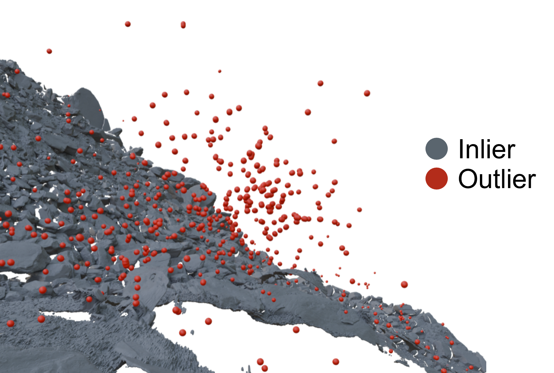
As shown in this example, points and point clusters that are detached from the surface are mostly considered outliers.
sor_k = 8
sor_std_dev_multiplier = 1.0
sor_remove_points = False

sor_epoch, inlier_outlier = py4dgeo.statistical_outlier_removal(
    epoch=voxel_epoch,
    k=sor_k,
    std_dev_multiplier=sor_std_dev_multiplier,
    remove_points=sor_remove_points,
)

sor_inlier_mask = inlier_outlier == 0
sor_outlier_mask = inlier_outlier == 1

kept_points = sor_epoch.cloud[sor_inlier_mask]
removed_points = sor_epoch.cloud[sor_outlier_mask]
removed_fraction = removed_points.shape[0] / sor_epoch.cloud.shape[0]

sor_attributes = {
    f"inlier_outlier_{sor_k}": inlier_outlier,
}

print(f"Input points:            {sor_epoch.cloud.shape[0]:,}")
print(f"Kept points:             {kept_points.shape[0]:,}")
print(f"Flagged outliers:        {removed_points.shape[0]:,} ({removed_fraction:.2%})")
[2026-06-23 09:45:24][INFO] Building KDTree structure with leaf parameter 10
SOR threshold: 1.239
Input points:            50,575
Kept points:             43,108
Flagged outliers:        7,467 (14.76%)
We now visualize the SOR flags. Inliers are shown in grey and points flagged as outliers are highlighted in red.
fig = plt.figure(figsize=(8, 8))
plot_every_nth = 1
ax = fig.add_subplot(projection="3d")
ax.scatter(
    kept_points[:, 0][::plot_every_nth],
    kept_points[:, 1][::plot_every_nth],
    kept_points[:, 2][::plot_every_nth],
    s=5,
    c="0.7",
    label="kept",
)
if removed_points.shape[0] > 0:
    ax.scatter(
        removed_points[:, 0][::plot_every_nth],
        removed_points[:, 1][::plot_every_nth],
        removed_points[:, 2][::plot_every_nth],
        s=1,
        c="red",
        label="removed",
    )
ax.view_init(elev=30, azim=120)
ax.set_xlabel("X [m]")
ax.set_ylabel("Y [m]")
ax.set_zlabel("Z [m]")
ax.set_title("Statistical outlier removal")
ax.legend()
ax.set_aspect("equal", "box")
plt.show()

VAPC Occupancy Differences
py4dgeo.Vapc is a voxel-based point cloud processing tool. We already used VAPC above for density estimation and spatial subsampling. Here we use the same voxel representation for a first comparison of two PLS epochs.
This first step only asks whether a voxel is occupied in epoch 1, in epoch 2, or in both. It is useful as a quick screening step, especially when many epochs need to be checked (Tabernig et al., 2025).
voxel_size_occupancy = 0.75

vapc_epoch1 = py4dgeo.Vapc(epoch1, voxel_size=voxel_size_occupancy)
vapc_epoch2 = py4dgeo.Vapc(epoch2, voxel_size=voxel_size_occupancy)

occupancy_change = vapc_epoch1.delta_vapc(vapc_epoch2)
occupancy_type = occupancy_change.out["delta_vapc"]

only_epoch1 = occupancy_type == 1
only_epoch2 = occupancy_type == 2
occupied_both = occupancy_type == 3

print(f"Voxel size for occupancy comparison: {voxel_size_occupancy} m")
print(f"Only epoch 1:     {only_epoch1.sum():,} voxels")
print(f"Only epoch 2:     {only_epoch2.sum():,} voxels")
print(f"Occupied in both: {occupied_both.sum():,} voxels")
Voxel size for occupancy comparison: 0.75 m
Only epoch 1:     6,845 voxels
Only epoch 2:     5,431 voxels
Occupied in both: 75,688 voxels
The occupancy result is plotted as voxel centers. Blue voxels are occupied only in the first epoch, red voxels only in the second epoch, and transparent grey voxels provide stable context.
occupancy_colors = np.full(occupancy_type.shape, "#C7C7C73C", dtype=object)
occupancy_colors[only_epoch1] = "tab:blue"
occupancy_colors[only_epoch2] = "tab:red"

fig = plt.figure(figsize=(9, 8))
ax = fig.add_subplot(projection="3d")
ax.scatter(
    occupancy_change.epoch.cloud[:, 0],
    occupancy_change.epoch.cloud[:, 1],
    occupancy_change.epoch.cloud[:, 2],
    c=occupancy_colors,
    s=5,
    marker="s",
)

ax.set_xlabel("X [m]")
ax.set_ylabel("Y [m]")
ax.set_zlabel("Z [m]")
ax.set_title("VAPC occupancy comparison")
ax.set_aspect("equal", "box")
ax.view_init(elev=30, azim=120)

legend_handles = [
    plt.Line2D([0], [0], marker="s", color="w", label="only epoch 1", markerfacecolor="tab:blue", markersize=6),
    plt.Line2D([0], [0], marker="s", color="w", label="only epoch 2", markerfacecolor="tab:red", markersize=6),
    plt.Line2D([0], [0], marker="s", color="w", label="both epochs", markerfacecolor="#C7C7C73C", markersize=6),
]
ax.legend(handles=legend_handles, title="Voxel occupancy")
plt.show()

Interpreting Occupancy Differences
In this snow-covered scene, voxels occupied only in epoch 1 can indicate places where snow was removed between the two scans. This may include snow melt, but also release and entrainment areas of an avalanche. Voxels occupied only in epoch 2 can indicate newly accumulated material, for example a deposition area. With the 0.75 m voxel size, we only see changes that are large enough to affect voxel occupancy.
This is still a coarse view. The plot does not provide detailed change magnitudes or a final event interpretation. Voxels occupied in both epochs remain shown as stable context here. If both epochs occupy the same voxel, the surface may still have changed inside that voxel. Distribution-based approaches such as VAPC Mahalanobis analysis are used for that step. Here it remains an outlook. Activity 3.3 introduces it on the rockfall study area.
References
- Lague, D., Brodu, N., & Leroux, J. (2013). Accurate 3D comparison of complex topography with terrestrial laser scanner: Application to the Rangitikei canyon (N-Z). ISPRS Journal of Photogrammetry and Remote Sensing, 82, pp. 10–26. doi: 10.1016/j.isprsjprs.2013.04.009.
- Tabernig, R., Albert, W., Weiser, H., & Höfle, B. (2025). A hierarchical approach for near real-time 3D surface change analysis of permanent laser scanning point clouds. In: 6th Joint International Symposium on Deformation Monitoring (JISDM). doi: 10.5445/IR/1000180377.