Time series-based methods of surface dynamics change analysis¶

In this tutorial, we will look at two different methods of time series-based analysis of 4D point clouds with time series clustering (Kuschnerus et al., 2021) and the extraction of 4D objects-by-change (Anders et al., 2021). For this, we will use a hands-on analysis example to learn how time series-based analysis can be performed.

Learning Objectives:¶

• Understand and apply time series analysis concepts to 4D point clouds.
• Use SpatiotemporalAnalysis to manage and process point cloud time series.
• Perform temporal smoothing to reduce noise in time series data.
• Apply k-means clustering to identify distinct change patterns.
• Use the 4D-OBC algorithm to extract and analyze individual change events.

Dataset¶

This activity uses the Schneeferner TLS point cloud time series from Activity 2, acquired at the Zugspitze, Germany. The sequence of epochs provides the input for time series change analysis with SpatiotemporalAnalysis, temporal smoothing, clustering, and 4D object extraction.

Setup and Data Loading¶

Our first step is to load a sequence of point clouds that were captured at different times. We will then calculate the M3C2 distances between each epoch and a selected reference epoch, respectively. The obtained time series of distances will be the basis for our further analysis.

In [1]:

from pathlib import Path
import py4dgeo
import numpy as np
from sklearn.cluster import KMeans
from datetime import datetime
import matplotlib as mpl
import matplotlib.pyplot as plt
import matplotlib.colors as mcolors
from scipy.spatial import ConvexHull
from matplotlib.patches import Polygon

from pathlib import Path import py4dgeo import numpy as np from sklearn.cluster import KMeans from datetime import datetime import matplotlib as mpl import matplotlib.pyplot as plt import matplotlib.colors as mcolors from scipy.spatial import ConvexHull from matplotlib.patches import Polygon

In the list of point cloud files you can see that we have one laz file per epoch available. The file name contains the timestamp of the epoch, respectively, in format YYMMDD_hhmmss. To use this information for our analysis, we read the timestamp information from the file names into datetime objects.

In [3]:

# specify the data path
data_path = Path("../data/activity_2/point_clouds")

all_files = list(data_path.glob("*.laz"))
pc_list = []
timestamps = []

for f in all_files:
    if not f.name.endswith('.laz'):
        continue
        
    parts = f.stem.split('_')
    if len(parts) >= 2 and parts[-2].isdigit() and len(parts[-2]) == 6 and parts[-1].isdigit() and len(parts[-1]) == 6:
        pc_list.append(f)
        timestamp_str = f"{parts[-2]}_{parts[-1]}"
        timestamp = datetime.strptime(timestamp_str, '%y%m%d_%H%M%S')
        timestamps.append(timestamp)

pc_list[:5] # print the first elements

# specify the data path data_path = Path("../data/activity_2/point_clouds") all_files = list(data_path.glob("*.laz")) pc_list = [] timestamps = [] for f in all_files: if not f.name.endswith('.laz'): continue parts = f.stem.split('_') if len(parts) >= 2 and parts[-2].isdigit() and len(parts[-2]) == 6 and parts[-1].isdigit() and len(parts[-1]) == 6: pc_list.append(f) timestamp_str = f"{parts[-2]}_{parts[-1]}" timestamp = datetime.strptime(timestamp_str, '%y%m%d_%H%M%S') timestamps.append(timestamp) pc_list[:5] # print the first elements

Out[3]:

[WindowsPath('../data/activity_2/point_clouds/schneeferner_180418_120027.laz'),
 WindowsPath('../data/activity_2/point_clouds/schneeferner_180418_130027.laz'),
 WindowsPath('../data/activity_2/point_clouds/schneeferner_180418_140027.laz'),
 WindowsPath('../data/activity_2/point_clouds/schneeferner_180418_150027.laz'),
 WindowsPath('../data/activity_2/point_clouds/schneeferner_180418_160023.laz')]

Now we use the point cloud files and timestamp information to create a SpatiotemporalAnalysis object, which is the main data structure for 3D time series in py4dgeo. The data object is backed by an archive file (zip), which needs to be specified when instantiating the object:

In [4]:

analysis = py4dgeo.SpatiotemporalAnalysis(f'{data_path}/schneeferner.zip', force=True)

analysis = py4dgeo.SpatiotemporalAnalysis(f'{data_path}/schneeferner.zip', force=True)

[2026-06-25 20:11:38][INFO] Creating analysis file ..\data\activity_2\point_clouds/schneeferner.zip

The concept of the py4dgeo SpatiotemporalAnalysis object is to add a time series of 3D point clouds in terms of their change values to one global reference epoch. These change values are derived for a set of core points using the M3C2 algorithm, which was introduced in py4dgeo in the activity of standard workflow. With each epoch added as M3C2 distances compared to the reference epoch, we also add the timestamp to be usable in time series analysis.

As reference epoch, we use the first epoch in our time series (i.e., list of point clouds):

In [ ]:

# specify the reference epoch
reference_epoch_file = pc_list[0]

# read the reference epoch and set the timestamp
reference_epoch = py4dgeo.read_from_las(reference_epoch_file)
reference_epoch.timestamp = timestamps[0]

# set the reference epoch in the spatiotemporal analysis object
analysis.reference_epoch = reference_epoch

# specify the reference epoch reference_epoch_file = pc_list[0] # read the reference epoch and set the timestamp reference_epoch = py4dgeo.read_from_las(reference_epoch_file) reference_epoch.timestamp = timestamps[0] # set the reference epoch in the spatiotemporal analysis object analysis.reference_epoch = reference_epoch

M3C2 distance calculation¶

For epochs to be added, we now configure the M3C2 algorithm to derive the change values.

In [ ]:

# specify corepoints, here all points of the reference epoch
analysis.corepoints = reference_epoch.cloud[::]

# specify M3C2 parameters
analysis.m3c2 = py4dgeo.M3C2(cyl_radius=1.0, normal_radii=(1.0,), max_distance=10.0, registration_error = 0.025)

# specify corepoints, here all points of the reference epoch analysis.corepoints = reference_epoch.cloud[::] # specify M3C2 parameters analysis.m3c2 = py4dgeo.M3C2(cyl_radius=1.0, normal_radii=(1.0,), max_distance=10.0, registration_error = 0.025)

Now we add all the other epochs with their timestamps. Note that we do not add every single epoch using the add_epochs() method, but compile a list of all epochs (limited only by available RAM). Adding them as entire batches saves a lot of processing time, as the analysis object needs to be re-configured in memory for each adding operation.

Please aware that this step may take a while.

In [ ]:

# create a list to collect epoch objects
epochs = []
# start from pc_list[1:] to skip the reference epoch
# since enumerate starts from 0, use timestamps[e+1] to match the epochs with their timestamps
for e, pc_file in enumerate(pc_list[1:]):
    epoch_file = pc_file
    epoch = py4dgeo.read_from_las(epoch_file)
    epoch.timestamp = timestamps[e+1]
    epochs.append(epoch)

# add epoch objects to the spatiotemporal analysis object
analysis.add_epochs(*epochs)

# create a list to collect epoch objects epochs = [] # start from pc_list[1:] to skip the reference epoch # since enumerate starts from 0, use timestamps[e+1] to match the epochs with their timestamps for e, pc_file in enumerate(pc_list[1:]): epoch_file = pc_file epoch = py4dgeo.read_from_las(epoch_file) epoch.timestamp = timestamps[e+1] epochs.append(epoch) # add epoch objects to the spatiotemporal analysis object analysis.add_epochs(*epochs)

Now we have a fully constructed spatiotemporal object, which contains the change values in the scene at each epoch, and the time series of surface changes at each core point location, along with all metadata.

In [8]:

# print the spatiotemporal analysis data for 3 corepoints and 5 epochs, respectively
print(f"Space-time distance array:\n{analysis.distances[:3,:5]}")
print(f"Uncertainties of M3C2 distance calculation:\n{analysis.uncertainties['lodetection'][:3, :5]}")
print(f"Timestamp deltas of analysis:\n{analysis.timedeltas[:5]}")

# print the spatiotemporal analysis data for 3 corepoints and 5 epochs, respectively print(f"Space-time distance array:\n{analysis.distances[:3,:5]}") print(f"Uncertainties of M3C2 distance calculation:\n{analysis.uncertainties['lodetection'][:3, :5]}") print(f"Timestamp deltas of analysis:\n{analysis.timedeltas[:5]}")

Space-time distance array:
[[-0.00090916 -0.0092291  -0.00523798  0.00357471 -0.01300597]
 [ 0.00472494 -0.00633247 -0.00151809  0.00078728 -0.01732864]
 [ 0.0026491  -0.01452403 -0.00742233 -0.00195866 -0.02317615]]
Uncertainties of M3C2 distance calculation:
[[0.05939054 0.05760474 0.06653623 0.05911205 0.06040037]
 [0.06383101 0.06259084 0.06683246 0.06625019 0.06283139]
 [0.06452989 0.06335329 0.06382436 0.06584868 0.06144326]]
Timestamp deltas of analysis:
[datetime.timedelta(seconds=3600), datetime.timedelta(seconds=7200), datetime.timedelta(seconds=10800), datetime.timedelta(seconds=14396), datetime.timedelta(seconds=19520)]

Visualization¶

We use these elements to visualize the changes in the scene for a selected epoch, together with the time series of surface changes at a selected location. The location here was selected separately in CloudCompare (as the corepoint id). You may select your own location coordinates or, in general, use external measurements, e.g., from GNSS, to look into a location of interest.

In [10]:

# create the figure
fig = plt.figure(figsize=(12, 5))
ax1 = fig.add_subplot(1, 2, 1, projection='3d', computed_zorder=False)
ax2 = fig.add_subplot(1, 2, 2)

# get the corepoints
corepoints = analysis.corepoints.cloud

# get change values of last epoch for all corepoints
distances = analysis.distances
distances_epoch = [d[100] for d in distances]

# get the time series of changes at a specific core point locations
cp_idx_sel = 62000
coord_sel = analysis.corepoints.cloud[cp_idx_sel]
timeseries_sel = distances[cp_idx_sel]

# get the list of timestamps from the reference epoch timestamp and timedeltas
timestamps = [t + analysis.reference_epoch.timestamp for t in analysis.timedeltas]

# plot the scene
d = ax1.scatter(corepoints[:,0], corepoints[:,1], corepoints[:,2], 
                c=distances_epoch[:], cmap='coolwarm_r', vmin=-1.5, vmax=1.5, s=1, zorder=1) 
plt.colorbar(d, format='%.2f', label='Distance [m]', ax=ax1, shrink=.5, pad=.15)

# add the location of the selected coordinate
ax1.scatter(coord_sel[0], coord_sel[1], coord_sel[2], c='black', s=3, zorder=2, label='Selected location')
ax1.legend()

# Prevent overlapping of axis labels and ticks
ax1.set_xlabel('X [m]', labelpad=20)
ax1.set_ylabel('Y [m]', labelpad=15)
ax1.set_zlabel('Z [m]', labelpad=10)

# Rotate tick labels to prevent overlap
ax1.tick_params(axis='x', labelrotation=45, pad=5)
ax1.tick_params(axis='y', labelrotation=-45, pad=5)
ax1.tick_params(axis='z', pad=5)

ax1.set_aspect('equal')
ax1.view_init(elev=30., azim=150.)

# Use modern f-string for title formatting
ax1.set_title(f'Changes at {analysis.reference_epoch.timestamp + analysis.timedeltas[100]}')

# plot the time series
ax2.plot(timestamps, timeseries_sel, color='blue')
ax2.set_xlabel('Date')
ax2.set_ylabel('Distance [m]')
ax2.grid()
ax2.set_ylim(-0.2, 1.0)
ax2.set_title('Time series at selected location')

plt.tight_layout()
plt.show()

# create the figure fig = plt.figure(figsize=(12, 5)) ax1 = fig.add_subplot(1, 2, 1, projection='3d', computed_zorder=False) ax2 = fig.add_subplot(1, 2, 2) # get the corepoints corepoints = analysis.corepoints.cloud # get change values of last epoch for all corepoints distances = analysis.distances distances_epoch = [d[100] for d in distances] # get the time series of changes at a specific core point locations cp_idx_sel = 62000 coord_sel = analysis.corepoints.cloud[cp_idx_sel] timeseries_sel = distances[cp_idx_sel] # get the list of timestamps from the reference epoch timestamp and timedeltas timestamps = [t + analysis.reference_epoch.timestamp for t in analysis.timedeltas] # plot the scene d = ax1.scatter(corepoints[:,0], corepoints[:,1], corepoints[:,2], c=distances_epoch[:], cmap='coolwarm_r', vmin=-1.5, vmax=1.5, s=1, zorder=1) plt.colorbar(d, format='%.2f', label='Distance [m]', ax=ax1, shrink=.5, pad=.15) # add the location of the selected coordinate ax1.scatter(coord_sel[0], coord_sel[1], coord_sel[2], c='black', s=3, zorder=2, label='Selected location') ax1.legend() # Prevent overlapping of axis labels and ticks ax1.set_xlabel('X [m]', labelpad=20) ax1.set_ylabel('Y [m]', labelpad=15) ax1.set_zlabel('Z [m]', labelpad=10) # Rotate tick labels to prevent overlap ax1.tick_params(axis='x', labelrotation=45, pad=5) ax1.tick_params(axis='y', labelrotation=-45, pad=5) ax1.tick_params(axis='z', pad=5) ax1.set_aspect('equal') ax1.view_init(elev=30., azim=150.) # Use modern f-string for title formatting ax1.set_title(f'Changes at {analysis.reference_epoch.timestamp + analysis.timedeltas[100]}') # plot the time series ax2.plot(timestamps, timeseries_sel, color='blue') ax2.set_xlabel('Date') ax2.set_ylabel('Distance [m]') ax2.grid() ax2.set_ylim(-0.2, 1.0) ax2.set_title('Time series at selected location') plt.tight_layout() plt.show()

Temporal smoothing¶

There are different approaches to spatiotemporal filtering. In our case, we already introduced spatial smoothing by applying the M3C2 to the point cloud epochs. We are therefore now using only time series averaging, to further filter the data in the temporal domain. We use a rolling median with a defined temporal window. For this, we use the temporal_averaging() function in py4dgeo.

In [11]:

analysis.smoothed_distances = py4dgeo.temporal_averaging(
    analysis.distances, smoothing_window=6
)

analysis.smoothed_distances = py4dgeo.temporal_averaging( analysis.distances, smoothing_window=6 )

[2026-06-25 20:16:33][INFO] Starting: Smoothing temporal data
[2026-06-25 20:16:52][INFO] Finished in 19.1179s: Smoothing temporal data

Now we can compare the raw and smoothed time series at our selected location:

In [12]:

# create the figure
fig, ax = plt.subplots(1,1,figsize=(7,5))

# plot the raw time series
ax.scatter(timestamps, timeseries_sel, color='blue', label='raw', s=5)

# plot the smoothed time series
timeseries_sel_smooth = analysis.smoothed_distances[cp_idx_sel]
ax.plot(timestamps, timeseries_sel_smooth, color='red', label='smooth')

ax.set_xlabel('Date')
ax.set_ylabel('Distance [m]')
ax.grid()
ax.set_ylim(-0.2,1.0)

plt.tight_layout()
plt.show()

# create the figure fig, ax = plt.subplots(1,1,figsize=(7,5)) # plot the raw time series ax.scatter(timestamps, timeseries_sel, color='blue', label='raw', s=5) # plot the smoothed time series timeseries_sel_smooth = analysis.smoothed_distances[cp_idx_sel] ax.plot(timestamps, timeseries_sel_smooth, color='red', label='smooth') ax.set_xlabel('Date') ax.set_ylabel('Distance [m]') ax.grid() ax.set_ylim(-0.2,1.0) plt.tight_layout() plt.show()

Time series clustering¶

Clustering of 3D time series is an approach developed to derive groups of similar change patterns in a scene, presented by Kuschnerus et al. (2021). As a method of unsupervised learning, it does not require to specify specific patterns or expected processes beforehand. This is ideal for near-continuous topographic observation, as we generally cannot know a priori about all possible types of surface activities occurring in the observed scene. The concept of time series clustering following Kuschnerus et al. (2021) is to group time series of a scene which exhibit a similar evolution of the topography throughout time. The objective is to separate the observed scene into distinct spatial regions where each region (cluster) represents a time series associated to a specific change pattern. This change pattern, ultimately, can be linked to characteristic surface processes shaping this region. The following figure visualizes how two time series in a scene can be similar according to their Euclidian distance (the lower, the more similar) or according to their correlation (between 0 and 1, with 1 being fully correlated):

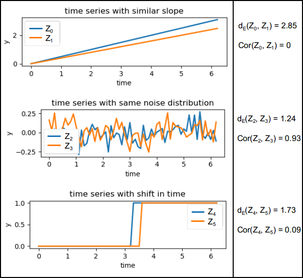
Example aspects how pairs of time series can be similar to one another according to Euclidian distance $d_E$ or correlation Cor. Figure by Kuschnerus et al. (2021) / CC BY 4.0.

Now that we have a time series of M3C2 distances for each core point, we can analyze the patterns of change. A powerful way to do this is through clustering. We hence perform time series clustering on our smoothed time series, looking into potential change patterns that may become visible. Following Kuschnerus et al. (2021), we apply a k-means clustering with a defined number of clusters, here k=5.

In [13]:

# use the smoothed distances for clustering
distances = analysis.smoothed_distances

# define the number of clusters
k=5

# create an array to store the labels
labels = np.full((distances.shape[0]), np.nan)

nan_indicator = np.logical_not(np.isnan(np.sum(distances, axis=1)))
kmeans = KMeans(n_clusters=k, random_state=0).fit(distances[nan_indicator, :])
labels[nan_indicator] = kmeans.labels_

# use the smoothed distances for clustering distances = analysis.smoothed_distances # define the number of clusters k=5 # create an array to store the labels labels = np.full((distances.shape[0]), np.nan) nan_indicator = np.logical_not(np.isnan(np.sum(distances, axis=1))) kmeans = KMeans(n_clusters=k, random_state=0).fit(distances[nan_indicator, :]) labels[nan_indicator] = kmeans.labels_

In [14]:

fig = plt.figure(figsize=(12, 5))
ax1 = fig.add_subplot(1, 2, 1, projection='3d', computed_zorder=False)
ax2 = fig.add_subplot(1, 2, 2)

corepoints = analysis.corepoints.cloud
d = ax1.scatter(corepoints[:, 0], corepoints[:, 1], corepoints[:, 2], c=labels, cmap='tab10', s=1)
ticks = np.arange(0, k, 1).astype(int)
cb = plt.colorbar(d, ticks=ticks, label='Cluster ID', ax=ax1, shrink=0.8, pad=0.15)

ax1.set_xlabel('Easting [m]', labelpad=15)
ax1.set_ylabel('Northing [m]', labelpad=15)
ax1.set_zlabel('Elevation [m]', labelpad=15) 
ax1.tick_params(axis='y', labelrotation=-45, pad=5)
ax1.view_init(elev=30., azim=150.)
ax1.set_aspect('equal') 

cmap_labels = labels / np.nanmax(labels)
cmap_clusters = mpl.colormaps['tab10']
labels_plotted = {}

for c in range(0, distances.shape[0], 100):
    ts = distances[c]
    label_curr = labels[c]
    if not label_curr in labels_plotted.keys():
        labels_plotted[label_curr] = [c]
    p1 = ax2.plot(timestamps, ts, c=cmap_clusters(cmap_labels[c]), linewidth=.5)
    
    labels_plotted[label_curr].append(c)

ax2.set_xlabel('Date')
ax2.set_ylabel('Distance [m]')
ax2.grid()

plt.tight_layout()
plt.show()

fig = plt.figure(figsize=(12, 5)) ax1 = fig.add_subplot(1, 2, 1, projection='3d', computed_zorder=False) ax2 = fig.add_subplot(1, 2, 2) corepoints = analysis.corepoints.cloud d = ax1.scatter(corepoints[:, 0], corepoints[:, 1], corepoints[:, 2], c=labels, cmap='tab10', s=1) ticks = np.arange(0, k, 1).astype(int) cb = plt.colorbar(d, ticks=ticks, label='Cluster ID', ax=ax1, shrink=0.8, pad=0.15) ax1.set_xlabel('Easting [m]', labelpad=15) ax1.set_ylabel('Northing [m]', labelpad=15) ax1.set_zlabel('Elevation [m]', labelpad=15) ax1.tick_params(axis='y', labelrotation=-45, pad=5) ax1.view_init(elev=30., azim=150.) ax1.set_aspect('equal') cmap_labels = labels / np.nanmax(labels) cmap_clusters = mpl.colormaps['tab10'] labels_plotted = {} for c in range(0, distances.shape[0], 100): ts = distances[c] label_curr = labels[c] if not label_curr in labels_plotted.keys(): labels_plotted[label_curr] = [c] p1 = ax2.plot(timestamps, ts, c=cmap_clusters(cmap_labels[c]), linewidth=.5) labels_plotted[label_curr].append(c) ax2.set_xlabel('Date') ax2.set_ylabel('Distance [m]') ax2.grid() plt.tight_layout() plt.show()

Extracting 4D-OBCs¶

Clustering helps us find regions with similar change patterns. However, sometimes we want to extract individual, discrete change events. This is where the 4D Objects-by-Change (4D-OBC) algorithm comes in.Therein, each objects represents a surface activity which occurs during a specific timespan (identified in the time series at a a location) and with a certain spatial extent (given by time series similarity in the local neighborhood during their timespan of occurrence). This method is implemented in py4dgeo with the two main steps of seed detection in the time series and spatial delineation using region growing based on the similarity of neighboring time series.

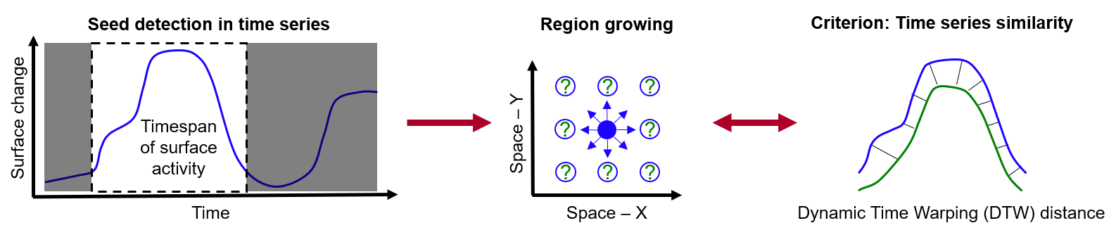
Main steps for the extraction of a 4D object-by-change with detection of a surface activity in the time series and subsequent region growing regarding the similarity of neighboring time series. Figure by K. Anders, following Anders et al. (2020).

In this example, we will not run the method for the entire scene, but extract one object at the selected location.

A powerful feature of py4dgeo is its flexibility. The core of the 4D-OBC method is the RegionGrowingAlgorithm, and its most critical step is the detection of "seed candidates" from which change objects grow. You can create your own seed detection strategy by inheriting from py4dgeo.segmentation.RegionGrowingAlgorithm. This allows you to tailor the algorithm to find specific types of changes that are most relevant to your application.
In our example of the snow-covered slope, we are looking for linear changes, such as the surface increase through avalanche deposition. As the original 4D-OBCs implemented in py4dgeo are targeting a different type of temporal process (see Anders et al., 2021), we define our own seed detection here.

In [16]:

from py4dgeo.segmentation import RegionGrowingSeed

class LinearChangeSeeds(py4dgeo.RegionGrowingAlgorithm):
    def find_seedpoints(self):

        # The list of generated seeds
        seeds = []

        # General seed criteria minimum magnitude and minimum timespan
        min_magn = self.height_threshold
        minperiod = self.minperiod
        maxperiod = 12

        # The list of core point indices to check as seeds
        if self.seed_candidates is None:
            # Use all corepoints if no selection specified, considering subsampling
            seed_candidates_curr = range(
                0, self.analysis.distances_for_compute.shape[0], self.seed_subsampling
                )
        else:
            # Use the specified corepoint indices, but consider subsampling
            seed_candidates_curr = self.seed_candidates[::self.seed_subsampling]

        # Interpolate nans in time series
        def interp_nan(data):
            bad_indexes = np.isnan(data)
            num_nans = len(np.argwhere(bad_indexes))
            num_not_nans = len(data) - num_nans
            if num_not_nans > 3:
                if num_nans > 0:
                    good_indexes = np.logical_not(bad_indexes)
                    good_data = data[good_indexes]
                    interpolated = np.interp(bad_indexes.nonzero()[0], good_indexes.nonzero()[0], good_data)
                    data[bad_indexes] = interpolated
            return data, num_nans, num_not_nans

        # Iterate over all time series to analyse their change points
        for cp_idx in seed_candidates_curr:

            timeseries = self.analysis.distances_for_compute[cp_idx, :]

            ts1d_interp, num_nans, num_not_nans = interp_nan(timeseries)
            if num_not_nans <= 3:
                continue

            # Use segment-wise linear regression to find change timespans
            from sklearn.tree import DecisionTreeRegressor
            from sklearn.linear_model import LinearRegression
            num_epochs = len(timeseries)
            xs = np.arange(0, num_epochs, dtype=float)

            dys = np.gradient(ts1d_interp, xs)

            rgr = DecisionTreeRegressor(max_depth=4) # depth controls the number of segments (sensitivity)
            rgr.fit(xs.reshape(-1, 1), dys.reshape(-1, 1))
            dys_dt = rgr.predict(xs.reshape(-1, 1)).flatten()

            ys_sl = np.ones(len(xs)) * np.nan            
            for y in np.unique(dys_dt):

                msk = dys_dt == y
                lin_reg = LinearRegression()
                lin_reg.fit(xs[msk].reshape(-1, 1), ts1d_interp[msk].reshape(-1, 1))
                ys_sl[msk] = lin_reg.predict(xs[msk].reshape(-1, 1)).flatten()
                x_vertices = [xs[msk][0], xs[msk][-1]]
                startn_det = int(round(x_vertices[0], 0))
                stopn_det = int(round(x_vertices[-1], 0))
                startp = np.max([startn_det - 1, 0])
                stopp = np.min([stopn_det + 1, len(timeseries) - 1])
                if (startp == 0) and stopp >= (len(timeseries) - 1):
                    continue

                # check minimum and maximum period criterion
                per = stopp - startp
                if (per < minperiod) or (per > maxperiod):
                    continue
                # check minimum magnitude criterion
                elif abs(np.max(timeseries[startp:stopp + 1]) - (np.min(timeseries[startp:stopp + 1]))) < min_magn:
                    continue
                # add seed
                else:
                    # construct the RegionGrowingSeed object consisting of index, start_epoch, end_epoch
                    curr_seed = RegionGrowingSeed(cp_idx, startp, stopp)
                    seeds.append(curr_seed)

        return seeds

from py4dgeo.segmentation import RegionGrowingSeed class LinearChangeSeeds(py4dgeo.RegionGrowingAlgorithm): def find_seedpoints(self): # The list of generated seeds seeds = [] # General seed criteria minimum magnitude and minimum timespan min_magn = self.height_threshold minperiod = self.minperiod maxperiod = 12 # The list of core point indices to check as seeds if self.seed_candidates is None: # Use all corepoints if no selection specified, considering subsampling seed_candidates_curr = range( 0, self.analysis.distances_for_compute.shape[0], self.seed_subsampling ) else: # Use the specified corepoint indices, but consider subsampling seed_candidates_curr = self.seed_candidates[::self.seed_subsampling] # Interpolate nans in time series def interp_nan(data): bad_indexes = np.isnan(data) num_nans = len(np.argwhere(bad_indexes)) num_not_nans = len(data) - num_nans if num_not_nans > 3: if num_nans > 0: good_indexes = np.logical_not(bad_indexes) good_data = data[good_indexes] interpolated = np.interp(bad_indexes.nonzero()[0], good_indexes.nonzero()[0], good_data) data[bad_indexes] = interpolated return data, num_nans, num_not_nans # Iterate over all time series to analyse their change points for cp_idx in seed_candidates_curr: timeseries = self.analysis.distances_for_compute[cp_idx, :] ts1d_interp, num_nans, num_not_nans = interp_nan(timeseries) if num_not_nans <= 3: continue # Use segment-wise linear regression to find change timespans from sklearn.tree import DecisionTreeRegressor from sklearn.linear_model import LinearRegression num_epochs = len(timeseries) xs = np.arange(0, num_epochs, dtype=float) dys = np.gradient(ts1d_interp, xs) rgr = DecisionTreeRegressor(max_depth=4) # depth controls the number of segments (sensitivity) rgr.fit(xs.reshape(-1, 1), dys.reshape(-1, 1)) dys_dt = rgr.predict(xs.reshape(-1, 1)).flatten() ys_sl = np.ones(len(xs)) * np.nan for y in np.unique(dys_dt): msk = dys_dt == y lin_reg = LinearRegression() lin_reg.fit(xs[msk].reshape(-1, 1), ts1d_interp[msk].reshape(-1, 1)) ys_sl[msk] = lin_reg.predict(xs[msk].reshape(-1, 1)).flatten() x_vertices = [xs[msk][0], xs[msk][-1]] startn_det = int(round(x_vertices[0], 0)) stopn_det = int(round(x_vertices[-1], 0)) startp = np.max([startn_det - 1, 0]) stopp = np.min([stopn_det + 1, len(timeseries) - 1]) if (startp == 0) and stopp >= (len(timeseries) - 1): continue # check minimum and maximum period criterion per = stopp - startp if (per < minperiod) or (per > maxperiod): continue # check minimum magnitude criterion elif abs(np.max(timeseries[startp:stopp + 1]) - (np.min(timeseries[startp:stopp + 1]))) < min_magn: continue # add seed else: # construct the RegionGrowingSeed object consisting of index, start_epoch, end_epoch curr_seed = RegionGrowingSeed(cp_idx, startp, stopp) seeds.append(curr_seed) return seeds

Next, we parametrize the 4D-OBC extraction by specifying a spatial neighborhood radius for searching locations during region growing, a minimum number of segments for an object to be valid (i.e. not discarded), and a minimum period and height threshold for seed timespans to be considered for region growing. The 4D-OBC workflow is encapsulated in the SpatiotemporalAnalysis class. Let's look at its key parameters:

• neighborhood_radius (float): Defines the radius for searching for neighboring points in space. This is fundamental to the region growing process, determining the extent of a point's local neighborhood.
• min_segments (int): The minimum number of points that a recognized region (or segment) must contain. This parameter filters out small, insignificant sets of points that are likely noise.
• minperiod (int): The minimum duration (in number of epochs) that a change event must persist. This helps to filter out transient, non-significant changes.
• height_threshold (float): The height (distance) threshold used during the seed detection process to determine if a change is significant. Only changes exceeding this threshold are considered potential starting points for a change event.
• thresholds (list of floats): A series of distance thresholds used during the region growing phase. The algorithm iterates through these thresholds from high to low, progressively relaxing the requirement for time series similarity to expand the extent of the change object.
• seed_candidates (list): A predefined list of point indices where the algorithm will exclusively look for seed points of change events. In this example, we restrict it to the single, previously selected point cp_idx_sel to extract an object only at that specific location.

In [17]:

# parametrize the 4D-OBC extraction
algo = LinearChangeSeeds(neighborhood_radius=1.0,
                         min_segments=50,
                         minperiod=2,
                         height_threshold=0.1,
                         thresholds=[0.5,0.6,0.7,0.8,0.9], seed_candidates=list([cp_idx_sel]))

# parametrize the 4D-OBC extraction algo = LinearChangeSeeds(neighborhood_radius=1.0, min_segments=50, minperiod=2, height_threshold=0.1, thresholds=[0.5,0.6,0.7,0.8,0.9], seed_candidates=list([cp_idx_sel]))

Finally, we simply run the method and the steps of seed detection and region growing are run automatically:

In [18]:

# run the algorithm
analysis.invalidate_results(seeds=True, objects=True, smoothed_distances=False) # only required if you want to re-run the algorithm
objects = algo.run(analysis)

# run the algorithm analysis.invalidate_results(seeds=True, objects=True, smoothed_distances=False) # only required if you want to re-run the algorithm objects = algo.run(analysis)

[2026-06-25 20:24:04][INFO] Removing intermediate results from the analysis file ..\data\activity_2\point_clouds/schneeferner.zip
[2026-06-25 20:24:04][INFO] Starting: Find seed candidates in time series
[2026-06-25 20:24:04][INFO] Finished in 0.0417s: Find seed candidates in time series
[2026-06-25 20:24:04][INFO] Starting: Sort seed candidates by priority
[2026-06-25 20:24:04][INFO] Finished in 0.0020s: Sort seed candidates by priority
[2026-06-25 20:24:04][INFO] Starting: Performing region growing on seed candidate 1/6
[2026-06-25 20:24:04][INFO] Finished in 0.0208s: Performing region growing on seed candidate 1/6
[2026-06-25 20:24:04][INFO] Starting: Performing region growing on seed candidate 2/6
[2026-06-25 20:24:04][INFO] Finished in 0.6046s: Performing region growing on seed candidate 2/6
[2026-06-25 20:24:04][INFO] Starting: Performing region growing on seed candidate 3/6
[2026-06-25 20:24:04][INFO] Finished in 0.0211s: Performing region growing on seed candidate 3/6
[2026-06-25 20:24:04][INFO] Starting: Performing region growing on seed candidate 6/6
[2026-06-25 20:24:04][INFO] Finished in 0.0113s: Performing region growing on seed candidate 6/6

Once finished, our SpatiotemporalAnalysis object holds all the information about the seeds and objects extracted for our analysis. Let's first have a look at the detected seeds (at the single time series of our selected location):

In [19]:

seed_timeseries = analysis.smoothed_distances[cp_idx_sel]
plt.plot(timestamps,seed_timeseries, c='black', linestyle='--', linewidth=0.5, label='Seed timeseries')

for sid, example_seed in enumerate(analysis.seeds):
    seed_end = example_seed.end_epoch
    seed_start = example_seed.start_epoch
    seed_cp_idx = example_seed.index

    plt.plot(timestamps[seed_start:seed_end+1], seed_timeseries[seed_start:seed_end+1], label=f'Seed {sid}')

plt.legend()
plt.show()

seed_timeseries = analysis.smoothed_distances[cp_idx_sel] plt.plot(timestamps,seed_timeseries, c='black', linestyle='--', linewidth=0.5, label='Seed timeseries') for sid, example_seed in enumerate(analysis.seeds): seed_end = example_seed.end_epoch seed_start = example_seed.start_epoch seed_cp_idx = example_seed.index plt.plot(timestamps[seed_start:seed_end+1], seed_timeseries[seed_start:seed_end+1], label=f'Seed {sid}') plt.legend() plt.show()

Several timespans of surface increase and decrease are detected, but we are only interested in the avalanche-related increase. Other seeds are found in the timespan of poor scan alignment (which we should leave out in our analysis, e.g., by not adding the epochs at all). We can now select the corresponding object to this seed and use a `plot()´ method to visualize the 4D-OBC by its time series (left) and in its spatial extent (right), colored by the time series similarity metric.

In [20]:

sel_seed_idx = 2
sel_seed = analysis.seeds[sel_seed_idx]
sel_object = analysis.objects[sel_seed_idx]

sel_object.plot()

sel_seed_idx = 2 sel_seed = analysis.seeds[sel_seed_idx] sel_object = analysis.objects[sel_seed_idx] sel_object.plot()

To better understand the object properties (time series behavior and spatial extent in the scene), we use the object data to visualize the change information:

In [21]:

fig, axs = plt.subplots(1, 2, figsize=(15, 5))
ax1, ax2 = axs

target_object = objects[sel_seed_idx]
idxs = target_object.indices
start_epoch = int(target_object.start_epoch)
epoch_of_interest = int(target_object.end_epoch)

distances_of_interest = analysis.smoothed_distances[:, epoch_of_interest]
magnitudes_of_interest = distances_of_interest - analysis.smoothed_distances[:, start_epoch]
crange = 1.0
cmap = mpl.colormaps['coolwarm_r'] 
norm = mcolors.CenteredNorm(halfrange=crange)
cmapvals = norm(magnitudes_of_interest)

for idx in idxs[::10]:
    ax1.plot(timestamps, analysis.smoothed_distances[idx], c=cmap(cmapvals[idx]), linewidth=0.5)

ax1.plot(timestamps, analysis.smoothed_distances[cp_idx_sel], c='black', linewidth=1.0, label='Seed timeseries')
ax1.axvspan(timestamps[start_epoch], timestamps[epoch_of_interest], 
            alpha=0.3, color='grey', label='4D-OBC timespan')

ax1.set_title('Time series of segmented 4D-OBC locations')
ax1.set_xlabel('Date')
ax1.set_ylabel('Distance [m]')
ax1.legend(loc='upper right')

cloud = analysis.corepoints.cloud
subset_cloud = cloud[idxs, :2]

sc = ax2.scatter(cloud[:, 0], cloud[:, 1], c=magnitudes_of_interest, 
                 cmap='coolwarm_r', vmin=-crange, vmax=crange, s=1)
plt.colorbar(sc, format='%.2f', label='Change magnitude [m]', ax=ax2)

hull = ConvexHull(subset_cloud)
ax2.add_patch(Polygon(subset_cloud[hull.vertices, 0:2], label='4D-OBC hull', fill=False, edgecolor='black'))

ax2.scatter(cloud[cp_idx_sel, 0], cloud[cp_idx_sel, 1], marker='*', c='black', s=50, label='Seed')
time_diff = timestamps[epoch_of_interest] - timestamps[start_epoch]
ax2.set_title(f'Magnitudes of change in the 4D-OBC timespan\n({time_diff} hours)')
ax2.set_xlabel('X [m]')
ax2.set_ylabel('Y [m]')
ax2.legend(loc='upper right')

plt.tight_layout()
plt.show()

fig, axs = plt.subplots(1, 2, figsize=(15, 5)) ax1, ax2 = axs target_object = objects[sel_seed_idx] idxs = target_object.indices start_epoch = int(target_object.start_epoch) epoch_of_interest = int(target_object.end_epoch) distances_of_interest = analysis.smoothed_distances[:, epoch_of_interest] magnitudes_of_interest = distances_of_interest - analysis.smoothed_distances[:, start_epoch] crange = 1.0 cmap = mpl.colormaps['coolwarm_r'] norm = mcolors.CenteredNorm(halfrange=crange) cmapvals = norm(magnitudes_of_interest) for idx in idxs[::10]: ax1.plot(timestamps, analysis.smoothed_distances[idx], c=cmap(cmapvals[idx]), linewidth=0.5) ax1.plot(timestamps, analysis.smoothed_distances[cp_idx_sel], c='black', linewidth=1.0, label='Seed timeseries') ax1.axvspan(timestamps[start_epoch], timestamps[epoch_of_interest], alpha=0.3, color='grey', label='4D-OBC timespan') ax1.set_title('Time series of segmented 4D-OBC locations') ax1.set_xlabel('Date') ax1.set_ylabel('Distance [m]') ax1.legend(loc='upper right') cloud = analysis.corepoints.cloud subset_cloud = cloud[idxs, :2] sc = ax2.scatter(cloud[:, 0], cloud[:, 1], c=magnitudes_of_interest, cmap='coolwarm_r', vmin=-crange, vmax=crange, s=1) plt.colorbar(sc, format='%.2f', label='Change magnitude [m]', ax=ax2) hull = ConvexHull(subset_cloud) ax2.add_patch(Polygon(subset_cloud[hull.vertices, 0:2], label='4D-OBC hull', fill=False, edgecolor='black')) ax2.scatter(cloud[cp_idx_sel, 0], cloud[cp_idx_sel, 1], marker='*', c='black', s=50, label='Seed') time_diff = timestamps[epoch_of_interest] - timestamps[start_epoch] ax2.set_title(f'Magnitudes of change in the 4D-OBC timespan\n({time_diff} hours)') ax2.set_xlabel('X [m]') ax2.set_ylabel('Y [m]') ax2.legend(loc='upper right') plt.tight_layout() plt.show()

References¶

• Anders, K., Lindenbergh, R. C., Vos, S. E., Mara, H., de Vries, S., & Höfle, B. (2019). High-Frequency 3D Geomorphic Observation Using Hourly Terrestrial Laser Scanning Data Of A Sandy Beach. ISPRS Ann. Photogramm. Remote Sens. Spatial Inf. Sci., IV-2/W5, pp. 317-324. doi: 10.5194/isprs-annals-IV-2-W5-317-2019.
• Anders, K., Winiwarter, L., Mara, H., Lindenbergh, R., Vos, S. E., & Höfle, B. (2021). Fully automatic spatiotemporal segmentation of 3D LiDAR time series for the extraction of natural surface changes. ISPRS Journal of Photogrammetry and Remote Sensing, 173, pp. 297-308. doi: 10.1016/j.isprsjprs.2021.01.015.
• Anders, K., Eberlein, S., & Höfle, B. (2022). Hourly Terrestrial Laser Scanning Point Clouds of Snow Cover in the Area of the Schneeferner, Zugspitze, Germany: PANGAEA. https://doi.org/10.1594/PANGAEA.941550.
• Kuschnerus, M., Lindenbergh, R., & Vos, S. (2021). Coastal change patterns from time series clustering of permanent laser scan data. Earth Surface Dynamics, 9 (1), pp. 89-103. doi: 10.5194/esurf-9-89-2021.