Monitoring deformation in a rockfall study area
In this activity, your task is to turn two TLS point clouds from before and after a rockfall into an interpretable deformation map. You will first check whether the two epochs are well aligned, then improve the registration if needed, and finally run M3C2 to identify where material was removed from the release area and where it was deposited. Along the way, you will test how core point spacing and normal radius affect the result, so that the final settings are not only correct but also efficient to compute.
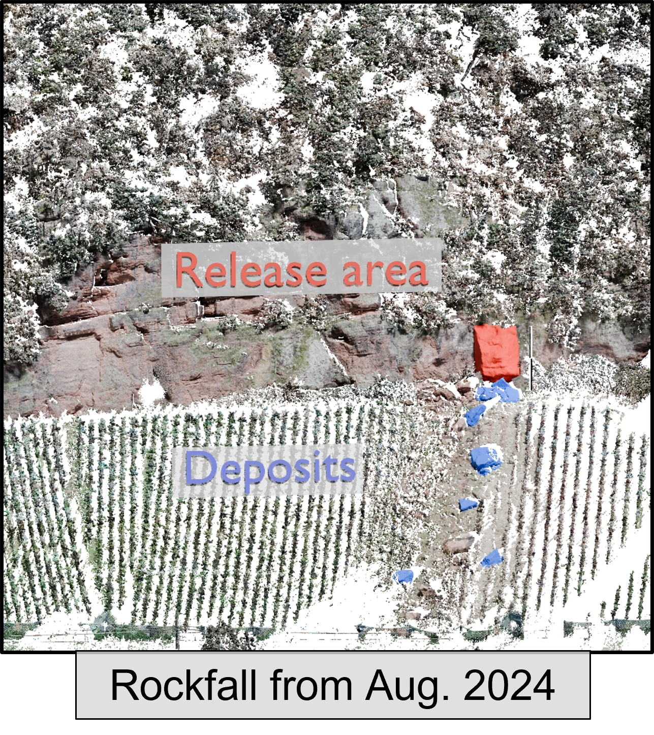
The figure shows the rock outcrop from the front. The red area marks the release area, where material was detached from the slope, and the blue areas mark the deposits. These are the surface changes that we want to detect in the point clouds.
Learning Objectives:
- Load a pair of TLS epochs for a deformation-monitoring case study.
- Check whether registration errors are present.
- Apply stable-area ICP before running the final change analysis.
- Choose voxel-based core point spacing and explain the trade-off between detail and runtime.
- Test M3C2 normal radius settings and compare their effect on full scene and release-area deformation patterns.
- Interpret which normal radius is selected by a multiscale M3C2 run.
Dataset
The test site is a rockfall-prone slope in Trier, Germany, monitored hourly with a permanently installed RIEGL VZ-2000i terrestrial laser scanner. The two point clouds used here were acquired one hour apart on August 26, 2024: one immediately before a rockfall of about 150 m³ and one immediately after it. A rockfall net stopped the detached material before it reached nearby transport infrastructure.
For this activity we treat the dataset as a bi-temporal change-detection problem. The workflow starts from the two TLS epochs, corrects their alignment, reduces the point density with voxel-based spatial subsampling, and then uses M3C2 (Lague et al., 2013) to map deformation in the full scene and in the release area.
Workflow
We use this workflow:
- Load the two TLS epochs of the rockfall study area.
- Run an initial registration preview to check whether the epochs are already well aligned.
- Register the unregistered target epoch with stable-area ICP.
- Use a zoomed registration check to compare the M3C2 distances before and after ICP.
- Inspect spatial subsampling at 1.0 m and 2.0 m voxel size.
- Run M3C2 at both core point resolutions, then compare normal radius settings and inspect the radius selected by the multiscale run.
Setup and Data Loading
We start by importing the required packages and disabling verbose py4dgeo tracing so that the notebook output stays focused on the analysis. The small helper below is used repeatedly for selecting zoom boxes.
from pathlib import Path
import py4dgeo
import numpy as np
import matplotlib.pyplot as plt
from matplotlib.colors import BoundaryNorm

# Keep the notebook output focused on the teaching result.
py4dgeo.enable_trace(False)
py4dgeo.enable_timeit(False)
# This function will later help us to select points inside a 3D zoom box for plotting or local analysis.
def points_in_zoom_box(cloud, center, size):
    half_size = np.asarray(size) / 2.0
    return np.all((cloud >= center - half_size) & (cloud <= center + half_size), axis=1)
Input data
As already mentioned, the input data are two terrestrial laser scanning epochs from a rockfall investigation area. The first epoch is used as the reference. The second epoch is intentionally loaded as an unregistered target so that the registration step remains visible in the workflow.
Besides the file paths, the scene-specific choices below are the zoom boxes used for the registration check and for the release-area interpretation. This will allow us to generate zoomed-in views in the plots.
data_path = Path("../data/activity_3_1_and_3_3/point_clouds")

reference_path = data_path / "ScanPos001 - SINGLESCANS - 240826_000005_registered.laz"
target_unregistered_path = data_path / "ScanPos001 - SINGLESCANS - 240826_010006_unregistered.laz"

reference_epoch = py4dgeo.read_from_las(reference_path)
target_unregistered = py4dgeo.read_from_las(target_unregistered_path)

print(f"Reference points: {reference_epoch.cloud.shape[0]:,}")
print(f"Target points:    {target_unregistered.cloud.shape[0]:,}")
Initial registration preview
Before estimating an ICP transformation, we run a coarse M3C2 comparison and inspect a zoom box where the registration offset is easy to see. This is intentionally a quick diagnostic rather than the final change analysis. The core points are spaced coarsely so that the calculation stays manageable, but the result is still good enough to show whether the two epochs are shifted relative to each other.
This cell may still compute for a little while.
# Settings for M3C2 preview.
preview_voxel_size = 1.0
preview_normal_radius = 2.5

# Settings for the zoom boxes.
registration_zoom_center = np.array([157.0, 498.0, 174.0])
registration_zoom_size = np.array([20.0, 20.0, 20.0])
release_zoom_center = np.array([197.0, 498.0, 165.0])
release_zoom_size = np.array([20.0, 20.0, 20.0])

# Subsample core points.
preview_vapc = py4dgeo.Vapc(reference_epoch, voxel_size=preview_voxel_size)
preview_corepoints = preview_vapc.reduce_to_feature("closest_to_voxel_centers").epoch.cloud

print(f"Running low-resolution M3C2 before registration on {preview_corepoints.shape[0]:,} core points ...")
preview_m3c2 = py4dgeo.M3C2(
    epochs=(reference_epoch, target_unregistered),
    corepoints=preview_corepoints,
    cyl_radius=preview_voxel_size,
    normal_radii=[preview_normal_radius],
)
preview_distances, preview_uncertainties = preview_m3c2.run()

finite_preview = preview_distances[np.isfinite(preview_distances)]
preview_vmax = np.nanpercentile(np.abs(finite_preview), 98) if finite_preview.size else 1.0
preview_vmax = max(preview_vmax, 0.01)
Before we move on, we define some helper functions that allow us to reuse certain parts of the code and make plotting easier.
# Draw the selected zoom box in a 3D plot.
def draw_zoom_box(ax, center, size, color="gold", linewidth=2.0, label="zoom box"):
    import matplotlib.patheffects as pe

    center = np.asarray(center)
    half_size = np.asarray(size) / 2.0
    corners = np.array([
        center + np.array([sx, sy, sz]) * half_size
        for sx in (-1, 1)
        for sy in (-1, 1)
        for sz in (-1, 1)
    ])
    edges = [
        (0, 1), (0, 2), (0, 4),
        (3, 1), (3, 2), (3, 7),
        (5, 1), (5, 4), (5, 7),
        (6, 2), (6, 4), (6, 7),
    ]

    for edge_index, (start, end) in enumerate(edges):
        line, = ax.plot(
            corners[[start, end], 0],
            corners[[start, end], 1],
            corners[[start, end], 2],
            color=color,
            linewidth=linewidth,
            linestyle="--",
            label=label if edge_index == 0 else None,
            zorder=20,
        )
        line.set_path_effects([
            pe.Stroke(linewidth=linewidth + 2.5, foreground="black"),
            pe.Normal(),
        ])

    ax.scatter(
        corners[:, 0],
        corners[:, 1],
        corners[:, 2],
        c=color,
        edgecolors="black",
        linewidths=0.5,
        s=18,
        depthshade=False,
        zorder=21,
    )


# Apply common labels, title, and equal aspect ratio to 3D axes.
def format_3d_axis(ax, title=None):
    if title is not None:
        ax.set_title(title)
    ax.set_xlabel("X [m]")
    ax.set_ylabel("Y [m]")
    ax.set_zlabel("Z [m]")
    ax.set_aspect("equal", "box")


# Plot core points colored by M3C2 distance with a fixed color scale.
def plot_m3c2_distances(ax, corepoints, distances, title, vmax, max_points=100_000, s=1):
    finite = np.isfinite(distances)
    plot_corepoints = corepoints[finite]
    plot_distances = distances[finite]
    plot_step = max(1, plot_corepoints.shape[0] // max_points)

    sc = ax.scatter(
        plot_corepoints[:, 0][::plot_step],
        plot_corepoints[:, 1][::plot_step],
        plot_corepoints[:, 2][::plot_step],
        c=plot_distances[::plot_step],
        cmap="coolwarm_r",
        s=s,
        vmin=-vmax,
        vmax=vmax,
    )
    format_3d_axis(ax, title)  # uses format_3d_axis() defined above
    return sc


# Plot reference and target points together inside the same zoom box.
def plot_two_clouds_in_zoom_box(
    ax,
    reference_cloud,
    target_cloud,
    center,
    size,
    reference_label="reference",
    target_label="target",
    reference_color="0.7",
    target_color="red",
    max_points=50_000,
):
    reference_zoom = reference_cloud[points_in_zoom_box(reference_cloud, center=center, size=size)]  # uses points_in_zoom_box() defined above
    target_zoom = target_cloud[points_in_zoom_box(target_cloud, center=center, size=size)]
    reference_step = max(1, reference_zoom.shape[0] // max_points)
    target_step = max(1, target_zoom.shape[0] // max_points)

    ax.scatter(
        reference_zoom[:, 0][::reference_step],
        reference_zoom[:, 1][::reference_step],
        reference_zoom[:, 2][::reference_step],
        c=reference_color,
        s=1,
        label=reference_label,
    )
    ax.scatter(
        target_zoom[:, 0][::target_step],
        target_zoom[:, 1][::target_step],
        target_zoom[:, 2][::target_step],
        c=target_color,
        s=1,
        label=target_label,
    )
    format_3d_axis(ax, "Registration-check zoom box")  # uses format_3d_axis() defined above
    ax.legend(markerscale=6)
The following figure has two parts. On the left, the reference points are colored by M3C2 distance. Red indicates negative distances, blue indicates positive distances, and values close to zero should appear close to white in the center of the color scale. Strong red or blue patterns in areas that should be stable can indicate that a registration offset is being measured as apparent surface change. On the right, the grey points are the reference epoch and the red points are the unregistered target epoch inside the same zoom box. This view helps to connect the distance pattern with the actual geometry of the two clouds.
# Plot the M3C2 result without coregistering the epochs.
fig = plt.figure(figsize=(13, 6), constrained_layout=True)
grid = fig.add_gridspec(1, 3, width_ratios=[1, 1, 0.04])

ax = fig.add_subplot(grid[0, 0], projection="3d")
ax.computed_zorder = False
sc = plot_m3c2_distances(  # uses plot_m3c2_distances() defined above
    ax,
    preview_corepoints,
    preview_distances,
    "Low-resolution M3C2 before registration",
    preview_vmax,
    s=2,
)
draw_zoom_box(  # uses draw_zoom_box() defined above
    ax,
    center=registration_zoom_center,
    size=registration_zoom_size,
    color="black",
    linewidth=0.5,
)
ax.legend(markerscale=6)

ax = fig.add_subplot(grid[0, 1], projection="3d")
plot_two_clouds_in_zoom_box(  # uses plot_two_clouds_in_zoom_box() defined above
    ax,
    reference_epoch.cloud[::2],
    target_unregistered.cloud[::2],
    center=registration_zoom_center,
    size=registration_zoom_size,
    target_label="unregistered target",
)

cbar = fig.colorbar(sc, cax=fig.add_subplot(grid[0, 2]))
cbar.set_label("M3C2 distance [m]")
plt.show()

As can be seen in the figure on the left, there are large positive and negative values, which appear to be divided by a line of minimal change from the lower left to the upper right. This suggests that the point cloud is not yet correctly aligned. The zoomed-in box view on the ''right'' further supports this, showing the ''systematic offset'' between the reference and the unregistered target.
Co-registration
We first align the unregistered target epoch to the reference epoch with stable-area ICP (Yang and Schwieger, 2023). The method estimates the transformation from parts of the scene that behave as unchanged surfaces, so the rockfall release and deposition areas should not dominate the registration.
The parameters can be set relative to the point spacing. We use 0.5 m registration subsampling below. The initial distance threshold is set to one voxel size, which is a practical upper bound for the expected coarse misalignment. The level of detection is set to 10 cm, between typical short- and longer-range TLS uncertainty. Supervoxels are built at five times the registration voxel size so that each local surface patch contains enough points for robust matching. Finally, normals are computed with 2.5 times the point spacing.
The stable-area ICP cell can compute for a little while because it estimates normals, builds stable-area supervoxels, and searches for corresponding surfaces.
If you are interested, vary the selected parameters and observe if and how the coregistration changes.
registration_voxel_size = 0.5
stable_area_initial_distance_threshold = registration_voxel_size
stable_area_level_of_detection = 10
stable_area_supervoxel_resolution = 5.0 * registration_voxel_size
stable_area_min_svp_num = 2
normal_radius = 2.5 * registration_voxel_size

reference_icp_vapc = py4dgeo.Vapc(reference_epoch, voxel_size=registration_voxel_size)
target_icp_vapc = py4dgeo.Vapc(target_unregistered, voxel_size=registration_voxel_size)

reference_icp = reference_icp_vapc.reduce_to_feature("closest_to_voxel_centers").epoch
target_icp = target_icp_vapc.reduce_to_feature("closest_to_voxel_centers").epoch

reference_icp.calculate_normals(radius = normal_radius)
target_icp.calculate_normals(radius = normal_radius)


print(f"Stable-area ICP voxel size:                  {registration_voxel_size} m")
print(f"Stable-area ICP initial distance threshold:  {stable_area_initial_distance_threshold} m")
print(f"Stable-area ICP level of detection:          {stable_area_level_of_detection} cm")
print(f"Stable-area ICP supervoxel resolution:       {stable_area_supervoxel_resolution} m")
print(f"Stable-area ICP reference subset:            {reference_icp.cloud.shape[0]:,} points")
print(f"Stable-area ICP target subset:               {target_icp.cloud.shape[0]:,} points")

stable_area_icp_trafo = py4dgeo.icp_with_stable_areas(
    reference_icp,
    target_icp,
    initial_distance_threshold=stable_area_initial_distance_threshold,
    level_of_detection=stable_area_level_of_detection,
    reference_supervoxel_resolution=stable_area_supervoxel_resolution,
    supervoxel_resolution=stable_area_supervoxel_resolution,
    min_svp_num=stable_area_min_svp_num,
    reduction_point=np.mean(reference_icp.cloud, axis=0),
)
target_stable_area_icp = py4dgeo.Epoch(target_unregistered.cloud.copy())
target_stable_area_icp.transform(stable_area_icp_trafo)

print("Stable-area ICP transformation estimated and applied to the target epoch.")
[2026-06-23 14:08:23][INFO] Building KDTree structure with leaf parameter 10
[2026-06-23 14:08:24][INFO] Starting: Calculating point cloud normals:
[2026-06-23 14:08:24][INFO] Finished in 0.0287s: Calculating point cloud normals:
[2026-06-23 14:08:24][INFO] Building KDTree structure with leaf parameter 10
[2026-06-23 14:08:24][INFO] Starting: Calculating point cloud normals:
[2026-06-23 14:08:24][INFO] Finished in 0.0293s: Calculating point cloud normals:
Stable-area ICP voxel size:                  0.5 m
Stable-area ICP initial distance threshold:  0.5 m
Stable-area ICP level of detection:          10 cm
Stable-area ICP supervoxel resolution:       2.5 m
Stable-area ICP reference subset:            188,976 points
Stable-area ICP target subset:               190,050 points
[2026-06-23 14:08:27][INFO] Initializing Epoch object from given point cloud
[2026-06-23 14:08:27][INFO] Building KDTree structure with leaf parameter 10
[2026-06-23 14:08:27][INFO] Initializing Epoch object from given point cloud
[2026-06-23 14:08:29][INFO] Initializing Epoch object from given point cloud
Stable-area ICP transformation estimated and applied to the target epoch.
Registration check
The plots below focus on the registration-check zoom box before and after stable-area ICP. We use the reference points inside this box as M3C2 core points and color them by M3C2 distance, so the local effect of the registration is visible directly. The same core points and the same M3C2 parameters are used in both panels. This is important because it means that the difference between the panels mainly comes from the registration step, not from a changed analysis setup.
In the left panel, before registration, coherent red or blue patches can appear even where no rockfall-related change is expected. This is the key point of the check: a registration error is spatially organized, not random. It often produces broad color patterns on stable surfaces because the whole target cloud is slightly shifted or rotated. With coolwarm_r, red shows negative distances and blue shows positive distances. In the right panel, after stable-area ICP, these stable parts should move closer to white or to smaller absolute distances. Real rockfall change can still remain visible elsewhere, but the stable surroundings should no longer dominate the interpretation.
# Lets start by extracting the points from zoom box
registration_check_corepoints = reference_epoch.cloud[
    points_in_zoom_box(reference_epoch.cloud, center=registration_zoom_center, size=registration_zoom_size)
]
if registration_check_corepoints.shape[0] == 0:
    raise ValueError("No reference points found in the registration-check zoom box.")


# Now we can compute M3C2 in the zoomed in area once on the dataset that was registered and once on the dataset that was not registered.
registration_check_parameters = {
    "cyl_radius": preview_voxel_size,
    "normal_radii": [preview_normal_radius],
}

registration_m3c2_results = {}
for label, target_epoch_for_check in [
    ("Before registration", target_unregistered),
    ("After registration", target_stable_area_icp),
]:
    print(f"Running zoomed M3C2 registration check ({label}) ...")
    registration_m3c2 = py4dgeo.M3C2(
        epochs=(reference_epoch, target_epoch_for_check),
        corepoints=registration_check_corepoints[::5],
        **registration_check_parameters,
    )
    distances, uncertainties = registration_m3c2.run()
    registration_m3c2_results[label] = {
        "distances": distances,
        "uncertainties": uncertainties,
    }
Running zoomed M3C2 registration check (Before registration) ...
Running zoomed M3C2 registration check (After registration) ...
[2026-06-23 14:08:31][INFO] Building KDTree structure with leaf parameter 10
# Now we can visualize the results easily using the already defined helper functions.
registration_vmax = 0.5
fig = plt.figure(figsize=(12, 6))
axes = []

for plot_idx, (label, result) in enumerate(registration_m3c2_results.items(), start=1):
    ax = fig.add_subplot(1, 2, plot_idx, projection="3d")
    axes.append(ax)
    sc = plot_m3c2_distances(
        ax,
        registration_check_corepoints[::5],
        result["distances"],
        label,
        registration_vmax,
        s=2,
    )

cbar = fig.colorbar(sc, ax=axes, shrink=0.65, pad=0.04)
cbar.set_label("M3C2 distance [m]")
fig.suptitle("Zoomed M3C2 registration check")
plt.show()

When we now compare the M3C2 distance before and after registration, it becomes apparent that, if we do not register the point clouds, we will falsely detect large deformations. After registration, however, it becomes clear that these deformations do not represent an actual change. Since we know that this zoomed area did not change between the epochs, we can conclude that registration was successful for this area. To ensure that the registration was successful globally and not only locally, it is recommended to search for multiple stable/unchanged areas distributed throughout a study site.
Spatial subsampling
We will now continue our investigation of the spatial subsampling at our rockfall study site. Using two different resolutions, we will first check how much the number of points is reduced, and secondly visually compare how these resolutions affect the point cloud representation of our study site.
For this first step we compare the two voxel sizes: 1.0 m and 2.0 m. The table printed below shows how many voxels are occupied and how many representative points remain after reducing each occupied voxel to one point.
The 1.0 m result keeps more spatial detail because more voxels are occupied and therefore more representative points remain. The 2.0 m result is much smaller and is therefore useful for quick tests runs. This is a typical trade-off in monitoring workflows: a dense set of core points can show smaller spatial details, but every following M3C2 run becomes more expensive.
The printed reduction factor is useful for judging runtime before starting the next tasks. If the number of retained points is much smaller, the following M3C2 calculations usually finish faster, but the final map will also be less detailed.
voxel_size_small = 1.0  # m
voxel_size_large = 2.0  # m
voxel_sizes = [voxel_size_small, voxel_size_large]

subsampling_results = {}
for voxel_size in voxel_sizes:
    vapc = py4dgeo.Vapc(reference_epoch, voxel_size=voxel_size)
    centers = vapc.compute_voxel_centers()
    counts = vapc.compute_features(["count"])["count"]
    reduced_epoch = vapc.reduce_to_feature("closest_to_voxel_centers").epoch

    subsampling_results[voxel_size] = {
        "centers": centers,
        "counts": counts,
        "epoch": reduced_epoch,
    }

    print(f"Reference epoch ({voxel_size:g} m voxels)")
    print(f"  occupied voxels:       {centers.shape[0]:,}")
    print(f"  reduced points:        {reduced_epoch.cloud.shape[0]:,}")
    print(f"  reduction factor:      {reference_epoch.cloud.shape[0] / max(reduced_epoch.cloud.shape[0], 1):.1f}x")
    print(f"  median points/voxel:   {np.nanmedian(counts):.1f}")
    print(f"  95% points/voxel:      {np.nanpercentile(counts, 95):.1f}")
    print()

corepoint_voxel_size = voxel_size_large
corepoints = subsampling_results[corepoint_voxel_size]["epoch"].cloud

print(f"M3C2 core points use the {corepoint_voxel_size:g} m subsampling: {corepoints.shape[0]:,} points")
Reference epoch (1 m voxels)
  occupied voxels:       61,062
  reduced points:        61,062
  reduction factor:      18.0x
  median points/voxel:   9.0
  95% points/voxel:      64.0

Reference epoch (2 m voxels)
  occupied voxels:       15,165
  reduced points:        15,165
  reduction factor:      72.3x
  median points/voxel:   38.0
  95% points/voxel:      254.0

M3C2 core points use the 2 m subsampling: 15,165 points
Spatial comparison
The next plot compares the original reference cloud with the two spatially subsampled versions inside the registration-check zoom box. This makes the reduction in point density visible before the subsampled points are used as M3C2 core points.
In the original cloud, many neighboring points describe the same local surface. After voxel-based subsampling, only one representative point is kept per occupied voxel. The 1.0 m version should still follow the local surface shape more closely, while the 2.0 m version looks more sparse and generalized. For M3C2 this means that distances are not computed everywhere, but at a regularized set of core points that represents the scene at the selected spatial resolution.
subsampling_plot_items = [
    ("Original", reference_epoch.cloud, "tab:grey"),
    (f"{voxel_size_small:g} m voxels", subsampling_results[voxel_size_small]["epoch"].cloud, "tab:blue"),
    (f"{voxel_size_large:g} m voxels", subsampling_results[voxel_size_large]["epoch"].cloud, "tab:orange"),
]

fig = plt.figure(figsize=(15, 5))

for plot_idx, (title, cloud, color) in enumerate(subsampling_plot_items, start=1):
    zoom_mask = points_in_zoom_box(cloud, center=registration_zoom_center, size=registration_zoom_size)
    ax = fig.add_subplot(1, len(subsampling_plot_items), plot_idx, projection="3d")
    zoom_cloud = cloud[zoom_mask]
    ax.scatter(zoom_cloud[:, 0], zoom_cloud[:, 1], zoom_cloud[:, 2], c=color, s=5)
    format_3d_axis(ax, f"{title}\n{zoom_cloud.shape[0]:,} points")  # uses format_3d_axis() defined above

fig.suptitle("Spatial subsampling in the registration-check zoom box")
plt.show()

Choosing the right M3C2 core point spacing
The next code cells compare 1.0 m and 2.0 m core point spacing with fixed M3C2 parameters. The aim is to see how much spatial detail is lost when the core points are coarser, and how much computation time can be saved. These M3C2 runs may take a little while, especially the 1.0 m run, because it uses more core points.
When you inspect the figure, compare the spatial pattern rather than individual points. The 1.0 m result should show a denser and more continuous deformation pattern. The 2.0 m result should show the same main rockfall signal if the spacing is still appropriate, but small details may disappear because fewer core points are available. Depending on how well the main rockfall signal is preserved, the point spacing should be chosen accordingly. This choice also depends on the specific use case and varies between study sites.
The color scale is kept the same in both panels. This allows a direct comparison of the distance magnitudes.
# Compare the effect of core point spacing while keeping the M3C2 parameters fixed.
basic_m3c2_settings = {
    "epochs": (reference_epoch, target_stable_area_icp),
    "cyl_radius": 3.0,
    "normal_radii": [3.0],
}

# Results will be stored here.
distances_by_label_spacing = {}
uncertainties_by_label_spacing = {}

# Coarser core point spacing.
basic_m3c2_settings["corepoints"] = subsampling_results[voxel_size_large]["epoch"].cloud
sparse_m3c2 = py4dgeo.M3C2(**basic_m3c2_settings)
sparse_distances, sparse_uncertainties = sparse_m3c2.run()
distances_by_label_spacing[voxel_size_large] = sparse_distances
uncertainties_by_label_spacing[voxel_size_large] = sparse_uncertainties
# Finer core point spacing.
basic_m3c2_settings["corepoints"] = subsampling_results[voxel_size_small]["epoch"].cloud
dense_m3c2 = py4dgeo.M3C2(**basic_m3c2_settings)
dense_distances, dense_uncertainties = dense_m3c2.run()
distances_by_label_spacing[voxel_size_small] = dense_distances
uncertainties_by_label_spacing[voxel_size_small] = dense_uncertainties

# The finer run contains more core points and therefore usually takes longer.
# Visualize the effect of core point spacing.
vmax = 1.0
vmin = -vmax

fig = plt.figure(figsize=(12, 6))
fig.subplots_adjust(right=0.86, wspace=0.05)
axes = []

for plot_idx, label in enumerate(distances_by_label_spacing, start=1):
    distances = distances_by_label_spacing[label]
    corepoints = subsampling_results[label]["epoch"].cloud
    ax = fig.add_subplot(1, len(distances_by_label_spacing), plot_idx, projection="3d")
    axes.append(ax)

    sc = ax.scatter(
        corepoints[:, 0],
        corepoints[:, 1],
        corepoints[:, 2],
        c=distances,
        cmap="coolwarm_r",
        s=1,
        vmin=vmin,
        vmax=vmax,
    )

    ax.set_xlabel("X [m]")
    ax.set_ylabel("Y [m]")
    ax.set_zlabel("Z [m]")
    ax.set_title(f"{label:g} m core point spacing")
    ax.set_aspect("equal", "box")

cbar_ax = fig.add_axes([0.95, 0.22, 0.02, 0.56])
cbar = fig.colorbar(sc, cax=cbar_ax)
cbar.set_label("M3C2 distance [m]")
fig.suptitle("M3C2 at different core point spacings")
plt.show()

Choosing the right M3C2 normal settings
The normal radius controls the scale at which M3C2 estimates the local surface orientation. With a small radius, the normal can react to small roughness elements and sharp local changes. This can be useful in a rough release area, but it can also make the result noisier. With a larger radius, the normal is estimated from a broader neighborhood. This often gives a smoother and more stable pattern, but it can average over small structures.
The next code cells compare normal_radius = 3 m, normal_radius = 6 m, and a multiscale combination of both radii at fixed 2.0 m core point spacing. These cells can compute for a little while because larger neighborhoods contain more points and therefore require more neighbor searches.
In the figure, look at whether the main deformation pattern stays in the same place for all settings. Then look at how sharp or smooth the pattern becomes. The same color scale is used here: red indicates negative distances, blue indicates positive distances, and white indicates little to no change. A useful parameter choice should keep the geomorphological signal visible without making stable areas look noisy.
# Compare the effect of normal radius while keeping the core points fixed.
basic_m3c2_settings = {
    "epochs": (reference_epoch, target_stable_area_icp),
    "corepoints": subsampling_results[voxel_size_large]["epoch"].cloud,
}

small_radius = 3.0
large_radius = 6.0

# Results will be stored here.
distances_by_label_radii = {}
uncertainties_by_label_radii = {}

# Single-scale run with the smaller normal radius.
basic_m3c2_settings["normal_radii"] = [small_radius]
basic_m3c2_settings["cyl_radius"] = small_radius
small_radius_m3c2 = py4dgeo.M3C2(**basic_m3c2_settings)
small_radius_distances, small_radius_uncertainties = small_radius_m3c2.run()
distances_by_label_radii[small_radius] = small_radius_distances
uncertainties_by_label_radii[small_radius] = small_radius_uncertainties
# Single-scale run with the larger normal radius.
basic_m3c2_settings["normal_radii"] = [large_radius]
basic_m3c2_settings["cyl_radius"] = large_radius
large_radius_m3c2 = py4dgeo.M3C2(**basic_m3c2_settings)
large_radius_distances, large_radius_uncertainties = large_radius_m3c2.run()
distances_by_label_radii[large_radius] = large_radius_distances
uncertainties_by_label_radii[large_radius] = large_radius_uncertainties

# While this is computing you can alread think about whether runtime increases more strongly when using more core points or larger radii.
# Multiscale run with both normal radii.
basic_m3c2_settings["cyl_radius"] = large_radius
basic_m3c2_settings["normal_radii"] = [small_radius, large_radius]
multi_radii_m3c2 = py4dgeo.M3C2(**basic_m3c2_settings)
multi_radii_distances, multi_radii_uncertainties = multi_radii_m3c2.run()
multiscale_label = f"{small_radius:g} and {large_radius:g}"
distances_by_label_radii[multiscale_label] = multi_radii_distances
uncertainties_by_label_radii[multiscale_label] = multi_radii_uncertainties
# Visualize the effect of normal radius.
vmax = 0.5
vmin = -vmax

fig = plt.figure(figsize=(12, 6))
fig.subplots_adjust(right=0.86, wspace=0.05)
axes = []

for plot_idx, label in enumerate(distances_by_label_radii, start=1):
    distances = distances_by_label_radii[label]
    corepoints = subsampling_results[voxel_size_large]["epoch"].cloud
    ax = fig.add_subplot(1, len(distances_by_label_radii), plot_idx, projection="3d")
    axes.append(ax)

    sc = ax.scatter(
        corepoints[:, 0],
        corepoints[:, 1],
        corepoints[:, 2],
        c=distances,
        cmap="coolwarm_r",
        s=2,
        vmin=vmin,
        vmax=vmax,
    )

    ax.set_xlabel("X [m]")
    ax.set_ylabel("Y [m]")
    ax.set_zlabel("Z [m]")
    ax.set_title(f"normal radius: {label} m")
    ax.set_aspect("equal", "box")

cbar_ax = fig.add_axes([0.95, 0.22, 0.02, 0.56])
cbar = fig.colorbar(sc, cax=cbar_ax)
cbar.set_label("M3C2 distance [m]")
fig.suptitle("M3C2 at different normal radii")
plt.show()

We now have three different deformation maps. The figure may create the impression that, when using multiple radii, only the larger radius was selected. This is not the case and the final part of this activity demonstrates how to visualise the selected radii.
Normal radius selected by the multiscale run
For the multiscale run, directions_radii() shows which normal radius was selected at each core point in the full scene. On the rock outcrop, smaller radii can preserve sharper local geometry, while larger radii smooth rough surfaces more strongly.
normal_radii_used = multi_radii_m3c2.directions_radii()
normal_radius_values = np.unique(normal_radii_used[np.isfinite(normal_radii_used)])

fig = plt.figure(figsize=(10,6))
ax = fig.add_subplot(111, projection="3d")

radius_cmap = plt.get_cmap("viridis", len(normal_radius_values))

if len(normal_radius_values) == 1:
    r = normal_radius_values[0]
    radius_boundaries = np.array([r - 0.5, r + 0.5])
else:
    radius_midpoints = (normal_radius_values[:-1] + normal_radius_values[1:]) / 2.0
    first_boundary = normal_radius_values[0] - (radius_midpoints[0] - normal_radius_values[0])
    last_boundary = normal_radius_values[-1] + (normal_radius_values[-1] - radius_midpoints[-1])
    radius_boundaries = np.concatenate([[first_boundary], radius_midpoints, [last_boundary]])

radius_norm = BoundaryNorm(radius_boundaries, radius_cmap.N)

sc = ax.scatter(
    corepoints[:, 0],
    corepoints[:, 1],
    corepoints[:, 2],
    c=normal_radii_used,
    s=1,
    cmap=radius_cmap,
    norm=radius_norm,
)

ax.set_box_aspect([
    np.ptp(corepoints[:, 0]),
    np.ptp(corepoints[:, 1]),
    np.ptp(corepoints[:, 2]),
])

cbar = fig.colorbar(
    sc,
    ax=ax,
    shrink=0.6,
    pad=0.1,
    ticks=normal_radius_values,
)

cbar.ax.set_yticklabels([str(radius) for radius in normal_radius_values])
cbar.set_label("selected normal radius [m]")

fig.suptitle("Full-scene multiscale M3C2 normal radius")
plt.show()

This final figure is not a deformation map. It is a parameter map. The colors show which normal radius the multiscale M3C2 run used locally. Since both radius values appear in the plot, the multiscale run did not simply behave like the single 6 m run everywhere. Instead, it selected different scales in different parts of the scene. This is useful to discuss because the deformation map alone does not show which local scale was chosen.
References
- Lague, D., Brodu, N., & Leroux, J. (2013). Accurate 3D comparison of complex topography with terrestrial laser scanner: Application to the Rangitikei canyon (N-Z). ISPRS Journal of Photogrammetry and Remote Sensing, 82, pp. 10-26. doi: 10.1016/j.isprsjprs.2013.04.009.
- Yang, Y., & Schwieger, V. (2023). Supervoxel-based targetless registration and identification of stable areas for deformed point clouds. Journal of Applied Geodesy, 17(2), pp. 161-170. doi: 10.1515/jag-2022-0031.