Monitoring of urban scene changes with airborne LiDAR time series
Change detection with py4dgeo is not limited to natural environments such as coastal beaches, glaciers, or rockfall slopes. The toolkit also applies well to urban scenes, where the landscape is driven by human activity. In these dynamic environments, buildings are constructed or demolished, vegetation grows or is removed, infrastructure is renewed, and the ground surface itself may subside or elevate due to construction activities.
Learning Objectives:
- Load the synthetic time series data.
- Run a simple bi-temporal M3C2 comparison between two epochs.
- Build a
SpatiotemporalAnalysiswith a reference epoch to compare a full time series. - Justify the M3C2 parameters (
cyl_radius,max_distance,registration_error) for the dataset. - Apply k-means clustering to identify urban change patterns.
Dataset
In this activity, we use a multi-temporal airborne laser scanning (ALS) dataset based on the publicly available AHN (Actueel Hoogtebestand Nederland) program, which provides nationwide LiDAR coverage of the Netherlands. The source tile (C_122000_488000) is located in Amsterdam and covers roughly 5 km × 6.25 km. For this tutorial we have cropped a smaller subarea of approximately 500 m × 500 m.
To effectively demonstrate continuous time series analysis, we have created a synthetic, temporally densified dataset. Using the real AHN3 (2014) and AHN5 (2023) epochs as our baseline, we synthetically interpolated the data to generate a high-frequency time series consisting of 30 epochs. For the change analysis below, we extract only the buildings from the scene and run M3C2 on these building point clouds, so that the analysis focuses on changes of the building stock (new constructions, demolitions, roof modifications) over the time series.
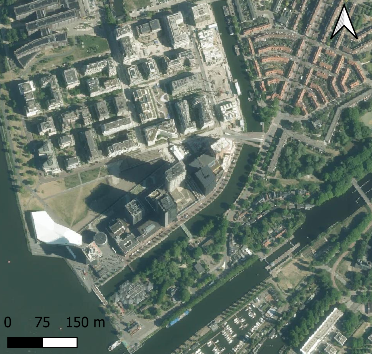
Aerial overview of the study area in Amsterdam. Aerial imagery sourced from PDOK, licensed under CC BY 4.0.
Setup and Data Loading
We start by importing the necessary libraries, assigning a virtual timestamp to each epoch, and reading all point clouds. Here, we assume a sampling frequency of 4 months between each epoch, starting from January 2014.
from pathlib import Path
import py4dgeo
import numpy as np
from datetime import datetime
import matplotlib as mpl
import matplotlib.pyplot as plt
import matplotlib.colors as colors
from sklearn.cluster import KMeans

# Keep the notebook output focused on the teaching result.
py4dgeo.enable_trace(False)
py4dgeo.enable_timeit(False)
data_path = Path("../data/activity_3_2/point_clouds")

file_list = [f for f in data_path.iterdir() if f.suffix == '.laz']
file_list = sorted(file_list, key=lambda x: int(''.join(filter(str.isdigit, x.stem))))

timestamps = []
for i in range(len(file_list)):
    # assuming each subsequent file is 4 months later
    total_months = i * 4
    new_year = 2014 + (total_months // 12)
    new_month = (total_months % 12) + 1
    timestamps.append(datetime(new_year, new_month, 1, 0, 0, 0))
Two ways to compare AHN data
There are two complementary workflows in py4dgeo for comparing these point clouds, and we will go through both:
Simple bi-temporal M3C2: compare two epochs directly with
py4dgeo.M3C2. This is the right tool when you only care about the change between a specific pair of epochs (e.g. "what changed between 2014 and 2023?"), and gives you a single distance map.SpatiotemporalAnalysistime series: register one epoch as the reference and add the remaining epochs as targets.py4dgeothen runs M3C2 between each target epoch and the reference, and stores the resulting distances as a time series per core point. This is the right tool when you want to study temporal patterns (smoothing, clustering, 4D objects).
We start by reading all epochs into memory once.
epochs = []
for filepath, timestamp in zip(file_list, timestamps):
    ep = py4dgeo.read_from_las(filepath)
    ep.timestamp = timestamp
    epochs.append(ep)
Bi-temporal analysis using M3C2
Let's visualize the first and last epoch to understand the urban scene.
fig, axes = plt.subplots(1, 2, figsize=(12,4))

# Plot Epoch 1
sc1 = axes[0].scatter(epochs[0].cloud[:, 0], epochs[0].cloud[:, 1],
                      c=epochs[0].cloud[:, 2], s=1, cmap='terrain')
axes[0].set_title(f'Epoch 1 ({timestamps[0].year}) - Elevation')
axes[0].axis('equal')

# Plot Epoch 30
sc2 = axes[1].scatter(epochs[29].cloud[:, 0], epochs[29].cloud[:, 1],
                      c=epochs[29].cloud[:, 2], s=1, cmap='terrain')
axes[1].set_title(f'Epoch 30 ({timestamps[29].year}) - Elevation')
axes[1].axis('equal')
for ax in axes:
    ax.set_aspect('equal')
    ax.set_xlabel('X [m]')
    ax.set_ylabel('Y [m]')
plt.colorbar(sc2, ax=axes.ravel().tolist(), label='Elevation (Z)')
plt.show()

We first compute change with the classical bi-temporal M3C2 algorithm directly between two epochs (the first and the last epoch, ~9 years). For this, we use the whole first epoch as our core points. Since urban changes (construction, demolition) are primarily vertical, we fix the M3C2 normal direction to (0, 0, 1). This avoids noise from local plane fitting and makes the result directly interpretable as vertical change. The other parameters are chosen to match the data characteristics: a cyl_radius of 2.0 m for robust averaging, a max_distance of 30.0 m to capture building-scale changes, and a registration_error of 5 cm.
corepoints = epochs[0].cloud
print(f'Corepoints: {corepoints.shape[0]:,} points')

# Bi-temporal M3C2 with normal forced to (0, 0, 1)
m3c2 = py4dgeo.M3C2(
    epochs=(epochs[0], epochs[29]),
    corepoints=corepoints,
    cyl_radius=2.0,
    max_distance=30.0,
    registration_error=0.05,
    corepoint_normals=np.tile([0, 0, 1], (corepoints.shape[0], 1))
)

distance, uncertainty = m3c2.run()
Corepoints: 37,597 points
[2026-06-25 22:11:45][INFO] Building KDTree structure with leaf parameter 10
[2026-06-25 22:11:45][INFO] Building KDTree structure with leaf parameter 10
Let's quickly look at the bi-temporal result. Large positive values (blue) indicate the surface is higher in 2023 than in 2014 (new buildings, raised ground, grown vegetation), and large negative values (red) indicate it is lower (demolitions, removed vegetation, excavations).
When observing the results, you might notice rings of large changes (red or blue) directly around the outlines of unchanged buildings, making them appear as if they are "growing" or shifting. This is a classic edge effect in point cloud comparisons. In urban scenes, airborne LiDAR point clouds often have occlusion, varying beam footprints, and slight variations in scanning angles between different flight campaigns. Furthermore, even with very small registration errors, a vertical wall might appear slightly offset between two epochs. When the M3C2 algorithm computes changes along a fixed vertical normal (0, 0, 1), these horizontal shifts at abrupt vertical edges translate into extreme (and often false) vertical elevation differences. Recognizing these artifacts is crucial for correctly interpreting change maps in built environments.
max_abs = np.nanmax(np.abs(distance))

fig, ax = plt.subplots(figsize=(7, 6))
sc = ax.scatter(corepoints[:, 0], corepoints[:, 1],
                c=distance, cmap='coolwarm_r', vmin=-max_abs, vmax=max_abs, s=1)
plt.colorbar(sc, ax=ax, label='M3C2 distance [m]', shrink=0.8)
ax.set_aspect('equal')
ax.set_xlabel('X [m]')
ax.set_ylabel('Y [m]')
ax.set_title('Bi-temporal M3C2')
plt.tight_layout()
plt.show()

Time series analysis
To analyse the change patterns across the entire 30-epoch time series, we use the SpatiotemporalAnalysis object. This is the right tool for time series analysis, as it calculates the M3C2 distances between a given reference epoch (here: the first epoch) and all subsequent epochs. We use the same core points and M3C2 parameters as in the bi-temporal workflow to ensure comparability. The analysis object is backed by a zip file, so all intermediate results are automatically saved.
# Create the analysis
analysis = py4dgeo.SpatiotemporalAnalysis(data_path/'dutch_urban.zip', force=True)
analysis.reference_epoch = epochs[0]
analysis.corepoints = corepoints

# Same M3C2 configuration as in Workflow 1 (including the fixed (0, 0, 1) normal)
analysis.m3c2 = py4dgeo.M3C2(
    cyl_radius=2.0,
    max_distance=30.0,
    registration_error=0.05,
    corepoint_normals=np.tile([0, 0, 1], (corepoints.shape[0], 1)),
)

analysis.add_epochs(*epochs)
[2026-06-25 22:11:46][INFO] Creating analysis file c:\rsa\project\py4dgeo_tutorial\test_py4dgeo_course\docs\notebooks\..\data\activity_3_2\point_clouds\dutch_urban.zip
[2026-06-25 22:11:46][INFO] Saving epoch to file 'C:\Users\93982\AppData\Local\Temp\tmpud4w92ql\reference_epoch.zip'
[2026-06-25 22:11:46][INFO] Saving a file without normals.
[2026-06-25 22:11:46][INFO] Initializing Epoch object from given point cloud
[2026-06-25 22:11:46][INFO] Building KDTree structure with leaf parameter 10
[2026-06-25 22:11:46][INFO] Saving epoch to file 'C:\Users\93982\AppData\Local\Temp\tmpmi21kmje\corepoints.zip'
[2026-06-25 22:11:46][INFO] Saving a file without normals.
[2026-06-25 22:11:46][INFO] Removing intermediate results from the analysis file c:\rsa\project\py4dgeo_tutorial\test_py4dgeo_course\docs\notebooks\..\data\activity_3_2\point_clouds\dutch_urban.zip
[2026-06-25 22:11:46][INFO] Starting: Adding epoch 1/30 to analysis object
[2026-06-25 22:11:47][INFO] Finished in 0.0643s: Adding epoch 1/30 to analysis object
[2026-06-25 22:11:47][INFO] Starting: Adding epoch 2/30 to analysis object
[2026-06-25 22:11:47][INFO] Building KDTree structure with leaf parameter 10
[2026-06-25 22:11:47][INFO] Finished in 0.1229s: Adding epoch 2/30 to analysis object
[2026-06-25 22:11:47][INFO] Starting: Adding epoch 3/30 to analysis object
[2026-06-25 22:11:47][INFO] Building KDTree structure with leaf parameter 10
[2026-06-25 22:11:47][INFO] Finished in 0.1307s: Adding epoch 3/30 to analysis object
[2026-06-25 22:11:47][INFO] Starting: Adding epoch 4/30 to analysis object
[2026-06-25 22:11:47][INFO] Building KDTree structure with leaf parameter 10
[2026-06-25 22:11:47][INFO] Finished in 0.1462s: Adding epoch 4/30 to analysis object
[2026-06-25 22:11:47][INFO] Starting: Adding epoch 5/30 to analysis object
[2026-06-25 22:11:47][INFO] Building KDTree structure with leaf parameter 10
[2026-06-25 22:11:47][INFO] Finished in 0.1394s: Adding epoch 5/30 to analysis object
[2026-06-25 22:11:47][INFO] Starting: Adding epoch 6/30 to analysis object
[2026-06-25 22:11:47][INFO] Building KDTree structure with leaf parameter 10
[2026-06-25 22:11:47][INFO] Finished in 0.1488s: Adding epoch 6/30 to analysis object
[2026-06-25 22:11:47][INFO] Starting: Adding epoch 7/30 to analysis object
[2026-06-25 22:11:47][INFO] Building KDTree structure with leaf parameter 10
[2026-06-25 22:11:47][INFO] Finished in 0.1611s: Adding epoch 7/30 to analysis object
[2026-06-25 22:11:47][INFO] Starting: Adding epoch 8/30 to analysis object
[2026-06-25 22:11:47][INFO] Building KDTree structure with leaf parameter 10
[2026-06-25 22:11:48][INFO] Finished in 0.1478s: Adding epoch 8/30 to analysis object
[2026-06-25 22:11:48][INFO] Starting: Adding epoch 9/30 to analysis object
[2026-06-25 22:11:48][INFO] Building KDTree structure with leaf parameter 10
[2026-06-25 22:11:48][INFO] Finished in 0.1530s: Adding epoch 9/30 to analysis object
[2026-06-25 22:11:48][INFO] Starting: Adding epoch 10/30 to analysis object
[2026-06-25 22:11:48][INFO] Building KDTree structure with leaf parameter 10
[2026-06-25 22:11:48][INFO] Finished in 0.1705s: Adding epoch 10/30 to analysis object
[2026-06-25 22:11:48][INFO] Starting: Adding epoch 11/30 to analysis object
[2026-06-25 22:11:48][INFO] Building KDTree structure with leaf parameter 10
[2026-06-25 22:11:48][INFO] Finished in 0.1678s: Adding epoch 11/30 to analysis object
[2026-06-25 22:11:48][INFO] Starting: Adding epoch 12/30 to analysis object
[2026-06-25 22:11:48][INFO] Building KDTree structure with leaf parameter 10
[2026-06-25 22:11:48][INFO] Finished in 0.1957s: Adding epoch 12/30 to analysis object
[2026-06-25 22:11:48][INFO] Starting: Adding epoch 13/30 to analysis object
[2026-06-25 22:11:48][INFO] Building KDTree structure with leaf parameter 10
[2026-06-25 22:11:48][INFO] Finished in 0.1593s: Adding epoch 13/30 to analysis object
[2026-06-25 22:11:48][INFO] Starting: Adding epoch 14/30 to analysis object
[2026-06-25 22:11:48][INFO] Building KDTree structure with leaf parameter 10
[2026-06-25 22:11:49][INFO] Finished in 0.2105s: Adding epoch 14/30 to analysis object
[2026-06-25 22:11:49][INFO] Starting: Adding epoch 15/30 to analysis object
[2026-06-25 22:11:49][INFO] Building KDTree structure with leaf parameter 10
[2026-06-25 22:11:49][INFO] Finished in 0.1586s: Adding epoch 15/30 to analysis object
[2026-06-25 22:11:49][INFO] Starting: Adding epoch 16/30 to analysis object
[2026-06-25 22:11:49][INFO] Building KDTree structure with leaf parameter 10
[2026-06-25 22:11:49][INFO] Finished in 0.2267s: Adding epoch 16/30 to analysis object
[2026-06-25 22:11:49][INFO] Starting: Adding epoch 17/30 to analysis object
[2026-06-25 22:11:49][INFO] Building KDTree structure with leaf parameter 10
[2026-06-25 22:11:49][INFO] Finished in 0.1932s: Adding epoch 17/30 to analysis object
[2026-06-25 22:11:49][INFO] Starting: Adding epoch 18/30 to analysis object
[2026-06-25 22:11:49][INFO] Building KDTree structure with leaf parameter 10
[2026-06-25 22:11:49][INFO] Finished in 0.2440s: Adding epoch 18/30 to analysis object
[2026-06-25 22:11:49][INFO] Starting: Adding epoch 19/30 to analysis object
[2026-06-25 22:11:49][INFO] Building KDTree structure with leaf parameter 10
[2026-06-25 22:11:50][INFO] Finished in 0.1877s: Adding epoch 19/30 to analysis object
[2026-06-25 22:11:50][INFO] Starting: Adding epoch 20/30 to analysis object
[2026-06-25 22:11:50][INFO] Building KDTree structure with leaf parameter 10
[2026-06-25 22:11:50][INFO] Finished in 0.1757s: Adding epoch 20/30 to analysis object
[2026-06-25 22:11:50][INFO] Starting: Adding epoch 21/30 to analysis object
[2026-06-25 22:11:50][INFO] Building KDTree structure with leaf parameter 10
[2026-06-25 22:11:50][INFO] Finished in 0.1727s: Adding epoch 21/30 to analysis object
[2026-06-25 22:11:50][INFO] Starting: Adding epoch 22/30 to analysis object
[2026-06-25 22:11:50][INFO] Building KDTree structure with leaf parameter 10
[2026-06-25 22:11:50][INFO] Finished in 0.1767s: Adding epoch 22/30 to analysis object
[2026-06-25 22:11:50][INFO] Starting: Adding epoch 23/30 to analysis object
[2026-06-25 22:11:50][INFO] Building KDTree structure with leaf parameter 10
[2026-06-25 22:11:50][INFO] Finished in 0.1619s: Adding epoch 23/30 to analysis object
[2026-06-25 22:11:50][INFO] Starting: Adding epoch 24/30 to analysis object
[2026-06-25 22:11:50][INFO] Building KDTree structure with leaf parameter 10
[2026-06-25 22:11:51][INFO] Finished in 0.1543s: Adding epoch 24/30 to analysis object
[2026-06-25 22:11:51][INFO] Starting: Adding epoch 25/30 to analysis object
[2026-06-25 22:11:51][INFO] Building KDTree structure with leaf parameter 10
[2026-06-25 22:11:51][INFO] Finished in 0.1538s: Adding epoch 25/30 to analysis object
[2026-06-25 22:11:51][INFO] Starting: Adding epoch 26/30 to analysis object
[2026-06-25 22:11:51][INFO] Building KDTree structure with leaf parameter 10
[2026-06-25 22:11:51][INFO] Finished in 0.1602s: Adding epoch 26/30 to analysis object
[2026-06-25 22:11:51][INFO] Starting: Adding epoch 27/30 to analysis object
[2026-06-25 22:11:51][INFO] Building KDTree structure with leaf parameter 10
[2026-06-25 22:11:51][INFO] Finished in 0.1905s: Adding epoch 27/30 to analysis object
[2026-06-25 22:11:51][INFO] Starting: Adding epoch 28/30 to analysis object
[2026-06-25 22:11:51][INFO] Building KDTree structure with leaf parameter 10
[2026-06-25 22:11:51][INFO] Finished in 0.1970s: Adding epoch 28/30 to analysis object
[2026-06-25 22:11:51][INFO] Starting: Adding epoch 29/30 to analysis object
[2026-06-25 22:11:51][INFO] Building KDTree structure with leaf parameter 10
[2026-06-25 22:11:51][INFO] Finished in 0.1603s: Adding epoch 29/30 to analysis object
[2026-06-25 22:11:51][INFO] Starting: Adding epoch 30/30 to analysis object
[2026-06-25 22:11:52][INFO] Finished in 0.1159s: Adding epoch 30/30 to analysis object
[2026-06-25 22:11:52][INFO] Starting: Rearranging space-time array in memory
[2026-06-25 22:11:54][INFO] Finished in 2.2954s: Rearranging space-time array in memory
[2026-06-25 22:11:54][INFO] Starting: Updating disk-based analysis archive with new epochs
[2026-06-25 22:11:54][INFO] Finished in 0.1912s: Updating disk-based analysis archive with new epochs
With the analysis built, we now have for each core point a time series of M3C2 distances relative to the reference epoch (here, the first epoch). Let us inspect the change map at the full time series at one selected core point. You can change cp_idx_sel to inspect a different location.
abs_timestamps = [analysis.reference_epoch.timestamp + dt for dt in analysis.timedeltas]
epoch_idx = analysis.distances.shape[1] - 1

# Find all corepoints that have a valid distance value at ALL epochs
valid_mask = ~np.isnan(analysis.distances).any(axis=1)
valid_indices = np.where(valid_mask)[0]

# Pick the one with the largest absolute change at the last epoch
abs_change_last_valid = np.abs(analysis.distances[valid_indices, epoch_idx])
selected_local_idx = np.argmax(abs_change_last_valid)
cp_idx_sel = valid_indices[selected_local_idx]
# cp_idx_sel = 12345  # Example: select a specific core point index (replace with actual index)

coord_sel = analysis.corepoints.cloud[cp_idx_sel]
print(f'Selected core point #{cp_idx_sel} at {coord_sel}, '
      f'change at last epoch = {analysis.distances[cp_idx_sel, epoch_idx]:.2f} m')
print(f'Time series values: {analysis.distances[cp_idx_sel]}')

fig = plt.figure(figsize=(13, 5))
ax1 = fig.add_subplot(1, 2, 1)
ax2 = fig.add_subplot(1, 2, 2)
cp = analysis.corepoints.cloud
max_abs = np.nanmax(np.abs(analysis.distances[:, epoch_idx]))
d = ax1.scatter(cp[:, 0], cp[:, 1],
                c=analysis.distances[:, epoch_idx],
                cmap='coolwarm_r', vmin=-max_abs, vmax=max_abs, s=1)
plt.colorbar(d, ax=ax1, label='M3C2 distance [m]', shrink=0.8)
ax1.scatter(coord_sel[0], coord_sel[1], c='black', s=100,
            marker='*', label='Selected location')
ax1.set_aspect('equal')
ax1.set_xlabel('X [m]')
ax1.set_ylabel('Y [m]')
ax1.set_title(f'Change {abs_timestamps[0].year} -> {abs_timestamps[epoch_idx].year}')
ax1.legend()
ax2.plot(abs_timestamps, analysis.distances[cp_idx_sel], 'o-', color='blue')
ax2.set_xlabel('Date')
ax2.set_ylabel('M3C2 distance [m]')
ax2.set_title('Time series at selected location')
ax2.grid()
fig.autofmt_xdate(rotation=45)
plt.tight_layout()
plt.show()
Selected core point #17751 at [-442.552628   285.747982    -3.3779765], change at last epoch = 29.92 m
Time series values: [ 0.          1.04269048  2.07835714  3.11457714  4.13945714  5.16914048
  6.20772381  7.25139714  8.27760714  9.29548571 10.33480714 11.38600714
 12.43183714 13.42848571 14.46647381 15.50354048 16.56483214 17.61333214
 18.57648571 19.62342857 20.66214048 21.71234048 22.73137381 23.74895714
 24.80470714 25.85325714 26.91190714 27.90737143 28.93518571 29.92397714]

Time series clustering
We then perform time series clustering on our time series, looking into potential change patterns that may become visible. Following Kuschnerus et al. (2021), we apply a k-means clustering with a defined number of clusters, here 4.
# use the distances for clustering
distances = analysis.distances

# define the number of clusters
k=4

labels = np.full((distances.shape[0]), np.nan)
nan_indicator = np.logical_not(np.isnan(np.sum(distances, axis=1)))
kmeans = KMeans(n_clusters=k, random_state=0).fit(distances[nan_indicator, :])
labels[nan_indicator] = kmeans.labels_
fig = plt.figure(figsize=(13, 5))
ax1 = fig.add_subplot(1, 2, 1, projection='3d', computed_zorder=False)
ax2 = fig.add_subplot(1, 2, 2)

base_cmap = mpl.colormaps['tab10'].resampled(k)
cmap_clusters = colors.ListedColormap([base_cmap(i) for i in range(k)])
norm_clusters = colors.BoundaryNorm(np.arange(-0.5, k, 1), cmap_clusters.N)

# get the corepoints
corepoints = analysis.corepoints.cloud

# plot the scene colored by cluster labels
d = ax1.scatter(corepoints[:, 0], corepoints[:, 1], corepoints[:, 2],
                c=labels, cmap=cmap_clusters, norm=norm_clusters, s=1)
ticks = np.arange(0, k, 1).astype(int)
cb = plt.colorbar(d, ticks=ticks, label='Cluster ID', ax=ax1, shrink=.7, pad=.15)

ax1.set_xlabel('X [m]', labelpad=10)
ax1.set_ylabel('Y [m]', labelpad=10)
ax1.set_zlabel('Z [m]', labelpad=4)

# Set a 1:1:1 aspect ratio based on the data ranges to avoid deformation
ax1.set_box_aspect((np.ptp(corepoints[:,0]), np.ptp(corepoints[:,1]), np.ptp(corepoints[:,2])))

ax1.locator_params(axis='x', nbins=4)
ax1.locator_params(axis='y', nbins=4)
ax1.locator_params(axis='z', nbins=1) # Use fewer ticks for the compressed Z axis
ax1.tick_params(axis='x', pad=0, labelsize=8)
ax1.tick_params(axis='y', pad=0, labelsize=8)
ax1.tick_params(axis='z', pad=0, labelsize=8)
ax1.view_init(elev=30., azim=150.)

# plot the time series colored by cluster labels (same coloring as the 3D scene)
labels_plotted = {}

# use only every 100th time series for plotting
for c in range(0, distances.shape[0], 100):
    ts = distances[c]
    label_curr = labels[c]
    if np.isnan(label_curr):
        continue
    if label_curr not in labels_plotted:
        labels_plotted[label_curr] = [c]
    p1 = ax2.plot(abs_timestamps, ts,
                  c=cmap_clusters(int(label_curr)),
                  label=label_curr, linewidth=.5)
    labels_plotted[label_curr].append(c)

ax2.set_xlabel('Date')
ax2.set_ylabel('Distance [m]')
ax2.grid()
fig.autofmt_xdate(rotation=45)
plt.tight_layout()
plt.show()

References
- Kuschnerus, M., Lindenbergh, R., & Vos, S. (2021). Coastal change patterns from time series clustering of permanent laser scan data. Earth Surface Dynamics, 9 (1), pp. 89-103. doi: 10.5194/esurf-9-89-2021.
- Lague, D., Brodu, N., & Leroux, J. (2013). Accurate 3D comparison of complex topography with terrestrial laser scanner: Application to the Rangitikei canyon (N-Z). ISPRS Journal of Photogrammetry and Remote Sensing, 82, pp. 10-26. doi: 10.1016/j.isprsjprs.2013.04.009.
- AHN — Actueel Hoogtebestand Nederland. National elevation product of the Netherlands. https://www.ahn.nl/
- PDOK. Luchtfoto 2025 Ortho 25cm RGB. https://www.pdok.nl/