Co-registration of point clouds
This tutorial demonstrates why co-registration is an essential preprocessing step for point cloud change analysis. We first run M3C2 on an intentionally unregistered epoch to inspect how registration errors can appear as false surface change. We then estimate a transformation matrix using the Iterative Closest Point (ICP) method, apply the transformation to the epoch, and repeat the M3C2 analysis on the same core points.
Learning Objectives:
- Understand why co-registration is required before comparing point clouds.
- Recognize how registration errors can appear as false surface change in M3C2 results.
- Estimate and apply a standard ICP transformation.
- Run M3C2 after registration and compare the result to the unregistered case.
- Interpret visual and distribution-based checks for registration improvement.
What is co-registration?
Co-registration is the process of aligning two point clouds before they are compared. Even if two datasets show the same scene, small shifts or rotations between them can be interpreted as surface change by change analysis methods.
This is particularly important because change analysis methods assume that the reference and target epochs are aligned. If the target epoch is displaced, these methods will measure part of that displacement as apparent topographic change. This can create false positives and make it difficult to distinguish actual surface change from registration artifacts.
What is ICP?
ICP (Iterative Closest Point) is a common algorithm for rigid point cloud registration (Besl and McKay, 1992). It repeatedly finds nearby point correspondences between a unregistered cloud and a fixed reference cloud, estimates the translation and rotation that best align those correspondences, and updates the unregistered cloud.
In this activity, the first epoch is used as the fixed reference and the second epoch is treated as the unregistered target.
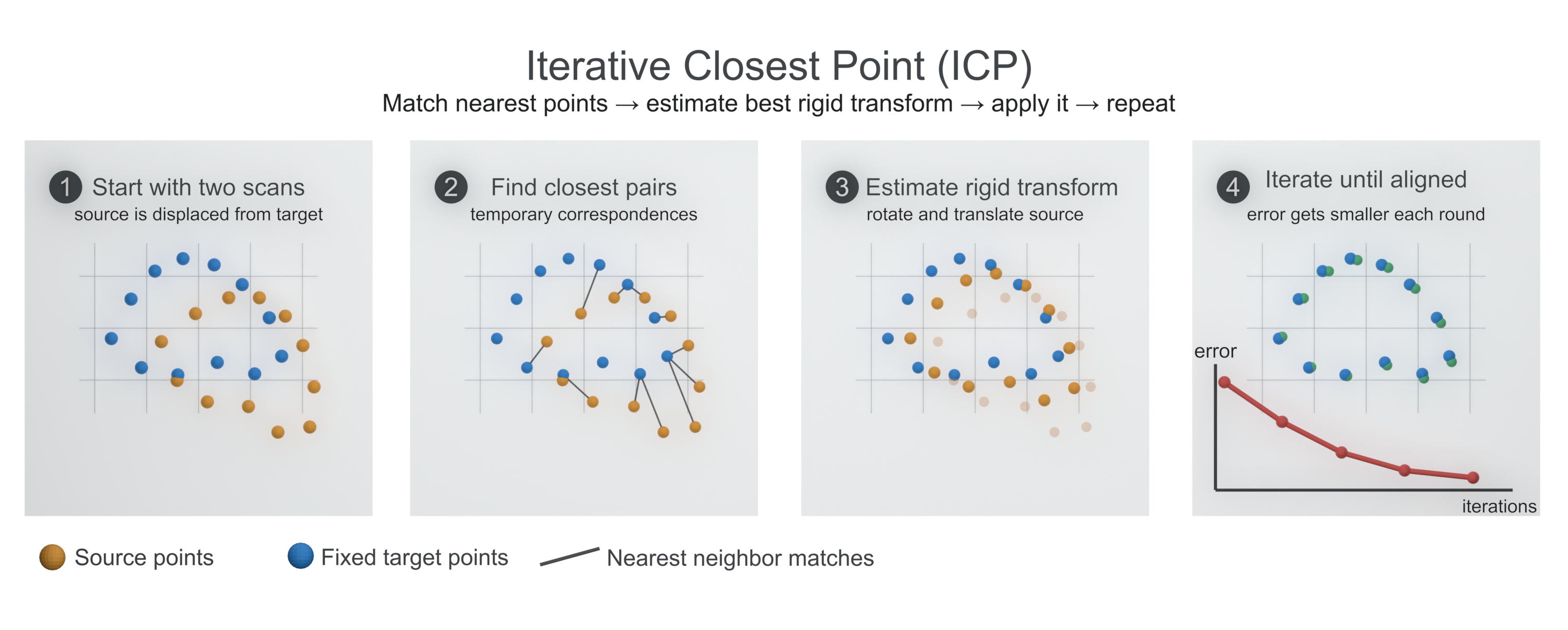
Schematic overview of the Iterative Closest Point (ICP) registration workflow: find nearest-neighbor correspondences, estimate a rigid transform, apply it, and iterate until alignment improves.
Setup and Data Loading
As in Activity 2.2, we import the required libraries.
from pathlib import Path
import py4dgeo
import numpy as np
import matplotlib.pyplot as plt

# Keep the notebook output focused on the teaching result.
py4dgeo.enable_trace(False)
py4dgeo.enable_timeit(False)
Now, we load two point cloud epochs that cover the same scene at two different points in time. The first epoch is already used as the reference. The second epoch is intentionally loaded in an unregistered state so that we can see how a misalignment affects the M3C2 result before we correct it.
data_path = Path("../data/activity_2/point_clouds")

reference_path = data_path / "schneeferner_180419_150005.laz"
unregistered_path = data_path / "schneeferner_180419_160005_unreg.laz"

reference_epoch = py4dgeo.read_from_las(reference_path)
unregistered_epoch = py4dgeo.read_from_las(unregistered_path)

print(f"Loaded reference epoch 1 with {reference_epoch.cloud.shape[0]:,} points.")
print(f"Loaded unregistered epoch 2 with {unregistered_epoch.cloud.shape[0]:,} points.")
M3C2 without registration
Before correcting the registration, we run M3C2 directly between the reference epoch and the unregistered target epoch. This is intentionally not the recommended workflow. The point is to inspect the type of result that can be produced when a registration error is interpreted as surface change.
As in Activity 2.2, the analysis is executed on so-called core points (Lague et al., 2013). To keep the computation short, we choose a subsampling by taking every 2nd point of the reference point cloud. The same core points and M3C2 parameters will later be reused after ICP registration.
# One core point every N reference points. Adjust for speed/detail.
corepoint_step = 2
corepoints = reference_epoch.cloud[::corepoint_step]

print(f"Using {corepoints.shape[0]:,} core points from {reference_epoch.cloud.shape[0]:,} reference points.")

m3c2_parameters = {
    "cyl_radius": 2.0,
    "normal_radii": [0.5, 1.0, 2.0],
}
Using 74,096 core points from 148,192 reference points.
print("Running M3C2 for unregistered target ...")
unregistered_m3c2 = py4dgeo.M3C2(
    epochs=(reference_epoch, unregistered_epoch),
    corepoints=corepoints,
    **m3c2_parameters,
)
unregistered_distances, unregistered_uncertainties = unregistered_m3c2.run()

vmax = 0.5
fig = plt.figure(figsize=(8, 6))
ax = fig.add_subplot(projection="3d")
sc = ax.scatter(
    corepoints[:, 0],
    corepoints[:, 1],
    corepoints[:, 2],
    c=unregistered_distances,
    cmap="coolwarm_r",
    s=1,
    vmin=-vmax,
    vmax=vmax,
)
cbar = plt.colorbar(sc, ax=ax, shrink=0.6, pad=0.12)
cbar.set_label("M3C2 distance [m]")
ax.set_xlabel("X [m]")
ax.set_ylabel("Y [m]")
ax.set_zlabel("Z [m]")
ax.set_title("M3C2 distances on core points without registration")
ax.set_aspect("equal", "box")
ax.view_init(elev=30, azim=120)
plt.show()
Running M3C2 for unregistered target ...
[2026-06-23 09:01:09][INFO] Building KDTree structure with leaf parameter 10
[2026-06-23 09:01:09][INFO] Building KDTree structure with leaf parameter 10

Standard ICP registration
Now we estimate a rigid transformation that aligns the moving target point cloud to the fixed reference point cloud. The standard ICP algorithm repeatedly finds nearest-neighbor correspondences, estimates a transformation from those correspondences, applies it internally, and checks whether the alignment improved.
Let's take a closer look at the inputs and parameters used below:
reference_icp: the fixed reference point cloud used for nearest-neighbor matching.unregistered_icp: the moving target point cloud that should be aligned to the reference.max_iterations=50: the maximum number of ICP refinement steps.tolerance=0.001: the convergence threshold. ICP stops early if the improvement between iterations becomes smaller than this value.
The standard ICP method assumes that most selected points represent stable geometry. This means that it may fail if large areas of the point cloud change between epochs, for example due to area-wide snowmelt or avalanches. To demonstrate the method, we have selected two subsequent epochs for which little change due to snowmelt is expected.
registration_step = 25  # Decrease for denser ICP input; increase for faster runtime.

reference_icp = py4dgeo.Epoch(reference_epoch.cloud[::registration_step].copy())
unregistered_icp = py4dgeo.Epoch(unregistered_epoch.cloud[::registration_step].copy())

print(f"ICP reference subset: {reference_icp.cloud.shape[0]:,} points")
print(f"ICP target subset:    {unregistered_icp.cloud.shape[0]:,} points")

standard_icp_trafo = py4dgeo.iterative_closest_point(
    reference_epoch=reference_icp,
    epoch=unregistered_icp,
    max_iterations=50,
    tolerance=0.001,
)

target_standard_icp = py4dgeo.Epoch(unregistered_epoch.cloud.copy())
target_standard_icp.transform(standard_icp_trafo)

print("Standard ICP transformation estimated and applied to the unregistered target copy.")
ICP reference subset: 5,928 points
ICP target subset:    5,928 points
[2026-06-23 09:01:14][INFO] Building KDTree structure with leaf parameter 10
Standard ICP transformation estimated and applied to the unregistered target copy.
M3C2 after ICP registration
Now we are ready to repeat the M3C2 calculation with the ICP-registered target epoch. The core points and M3C2 parameters remain the same as in the unregistered run, so the comparison focuses on the effect of registration rather than on a change in the analysis setup.
print("Running M3C2 after using standard ICP ...")
standard_icp_m3c2 = py4dgeo.M3C2(
    epochs=(reference_epoch, target_standard_icp),
    corepoints=corepoints,
    **m3c2_parameters,
)
standard_icp_distances, standard_icp_uncertainties = standard_icp_m3c2.run()

distances_by_label = {
    "unregistered": unregistered_distances,
    "standard ICP": standard_icp_distances,
}
uncertainties_by_label = {
    "unregistered": unregistered_uncertainties,
    "standard ICP": standard_icp_uncertainties,
}
Running M3C2 after using standard ICP ...
[2026-06-23 09:01:15][INFO] Building KDTree structure with leaf parameter 10
Visualization
Now that we have M3C2 distances for both cases, a fast way to interpret them is to visualize them on the point cloud. Following the same idea as in Activity 2.2, we plot the core points in 3D and use the M3C2 distances to color each point.
Here we place two 3D views next to each other so that the effect of registration can be compared directly:
- the unregistered target (left), and
- the target transformed with standard ICP (right).
We use a diverging colormap (coolwarm_r) with the same color scale for both plots:
- Blue indicates positive change, which is expected in the avalanche deposition area.
- Red indicates negative change, which can be expected from snowmelt, but also in the release and entrainment areas of an avalanche.
- White indicates little to no change.
We also set a threshold (vmax) to cap the color scale. This helps to highlight the main spatial pattern and prevents extreme outliers from dominating the visualization.
comparison_labels = ["unregistered", "standard ICP"]

# Use one symmetric color scale for both panels.
vmax = 0.5
vmin = -vmax

fig = plt.figure(figsize=(12, 6))
fig.subplots_adjust(right=0.86, wspace=0.05)
axes = []

for plot_idx, label in enumerate(comparison_labels, start=1):
    distances = distances_by_label[label]
    ax = fig.add_subplot(1, len(comparison_labels), plot_idx, projection="3d")
    axes.append(ax)

    sc = ax.scatter(
        corepoints[:, 0],
        corepoints[:, 1],
        corepoints[:, 2],
        c=distances,
        cmap="coolwarm_r",
        s=1,
        vmin=vmin,
        vmax=vmax,
    )

    ax.set_xlabel("X [m]")
    ax.set_ylabel("Y [m]")
    ax.set_zlabel("Z [m]")
    ax.set_title(label)
    ax.set_aspect("equal", "box")
    ax.view_init(elev=30, azim=120)

cbar_ax = fig.add_axes([0.95, 0.22, 0.02, 0.56])
cbar = fig.colorbar(sc, cax=cbar_ax)
cbar.set_label("M3C2 distance [m]")
fig.suptitle("M3C2 distances without and with standard ICP registration")
plt.show()

Registration error from stable areas
We can also estimate the registration error following the approach suggested by Fey and Wichmann (2017) and Zahs et al. (2022). The idea is to evaluate the remaining M3C2 distances in parts of the scene that are assumed to be stable. If these areas did not change, the remaining distances provide an empirical estimate of the registration error.
To achieve this, we manually select two areas in the stable surroundings of the unstable zone. We combine both stable areas into a single mask and calculate one standard deviation from all finite registered M3C2 distances in the selected stable areas. This value is used as the registration error estimate.
bbox_extent = 10  # m
stable_area_boxes = {
    "stable_area_1": {
        "xmin": -230 - bbox_extent,
        "xmax": -230 + bbox_extent,
        "ymin": 134 - bbox_extent,
        "ymax": 134 + bbox_extent,
        "zmin": -97 - bbox_extent,
        "zmax": -97 + bbox_extent,
    },
    "stable_area_2": {
        "xmin": 36 - bbox_extent,
        "xmax": 36 + bbox_extent,
        "ymin": 168 - bbox_extent,
        "ymax": 168 + bbox_extent,
        "zmin": 24.5 - bbox_extent,
        "zmax": 24.5 + bbox_extent,
    },
}

stable_area_mask = np.zeros(corepoints.shape[0], dtype=bool)

for label, box in stable_area_boxes.items():
    in_box = (
        (corepoints[:, 0] >= box["xmin"])
        & (corepoints[:, 0] <= box["xmax"])
        & (corepoints[:, 1] >= box["ymin"])
        & (corepoints[:, 1] <= box["ymax"])
        & (corepoints[:, 2] >= box["zmin"])
        & (corepoints[:, 2] <= box["zmax"])
    )
    stable_area_mask |= in_box

distances_in_stable_areas = standard_icp_distances[stable_area_mask]
distances_in_stable_areas = distances_in_stable_areas[np.isfinite(distances_in_stable_areas)]

if distances_in_stable_areas.size < 2:
    raise ValueError("The selected stable areas contain fewer than two finite M3C2 distances.")

registration_error = np.nanstd(distances_in_stable_areas, ddof=1)
print(f"Stable area core points: {distances_in_stable_areas.size}")
print(f"Registration error: {registration_error:.4f} m")
Stable area core points: 837
Registration error: 0.0130 m
Comparison of distance distribution with and without co-registration
The 3D visualisation showed where the differences occur. Histograms provide an additional view of the result by showing the overall distribution of M3C2 distances. After a successful registration, distances on stable parts of the scene should generally become more centered around zero, and the distribution should become narrower.
fig, ax = plt.subplots(figsize=(9, 5))
vmax = 1.0
bins = np.linspace(-vmax, vmax, 100)
distribution_stats = {}
for label, distances in distances_by_label.items():
    finite = distances[np.isfinite(distances)]
    mean = np.mean(finite)
    std = np.std(finite, ddof=1)
    distribution_stats[label] = {"mean": mean, "std": std}
    _, _, patches = ax.hist(
        finite,
        bins=bins,
        alpha=0.75,
        label=f"{label} distribution (std={std:.3f} m)",
        histtype="step",
        linewidth=2,
    )
    ax.axvline(
        mean,
        color=patches[0].get_edgecolor(),
        linestyle=":",
        linewidth=3,
        label=f"{label} mean={mean:.3f} m",
    )

mean_shift = (
    distribution_stats["standard ICP"]["mean"]
    - distribution_stats["unregistered"]["mean"]
)
ax.text(
    0.72,
    0.98,
    f"Mean shift after ICP: {mean_shift:+.3f} m",
    transform=ax.transAxes,
    va="top",
    bbox={"boxstyle": "round", "facecolor": "white", "alpha": 0.8},
)

ax.axvline(0, color="black", linewidth=1)
ax.set_xlabel("M3C2 distance [m]")
ax.set_ylabel("Number of core points")
ax.set_title("Distance distribution without and with standard ICP registration")
ax.legend()
plt.tight_layout()
plt.show()

Standard ICP is only one registration option. It can be biased when changed areas contribute strongly to the transformation estimate. In Activity 3.1, we will continue with further registration algorithms, specifically the stable-area ICP, which estimates the transformation from stable parts of the scene instead of from the full changed scene.
References
- Lague, D., Brodu, N., & Leroux, J. (2013). Accurate 3D comparison of complex topography with terrestrial laser scanner: Application to the Rangitikei canyon (N-Z). ISPRS Journal of Photogrammetry and Remote Sensing, 82, pp. 10–26. doi: 10.1016/j.isprsjprs.2013.04.009.
- Besl, P. J., & McKay, N. D. (1992). A method for registration of 3-D shapes. IEEE Transactions on Pattern Analysis and Machine Intelligence, 14(2), pp. 239–256. doi: 10.1109/34.121791.
- Fey, C., & Wichmann, V. (2017). Long-range terrestrial laser scanning for geomorphological change detection in alpine terrain - handling uncertainties. Earth Surface Processes and Landforms, 42(5), pp. 789–802. doi: 10.1002/esp.4022.
- Zahs, V., Winiwarter, L., Anders, K., Williams, J. G., Rutzinger, M., & Hoefle, B. (2022). Correspondence-driven plane-based M3C2 for lower uncertainty in 3D topographic change quantification. ISPRS Journal of Photogrammetry and Remote Sensing, 183, pp. 541–559. doi: 10.1016/j.isprsjprs.2021.11.018.