Distinguishing between relevant and non-relevant changes
This notebook continues the voxel-based idea from Activity 2.4 for the Trier rockfall study area. Activity 2.4 stops at the coarse occupancy comparison. Here, we use the shared occupied voxels for a first hierarchical change analysis of potentially relevant and non-relevant changes. The task is to reduce the scene to candidate areas, then check how point-based M3C2 analysis can be conducted in these reduced areas, and how we can achive this without losing the relevant rockfall signal.
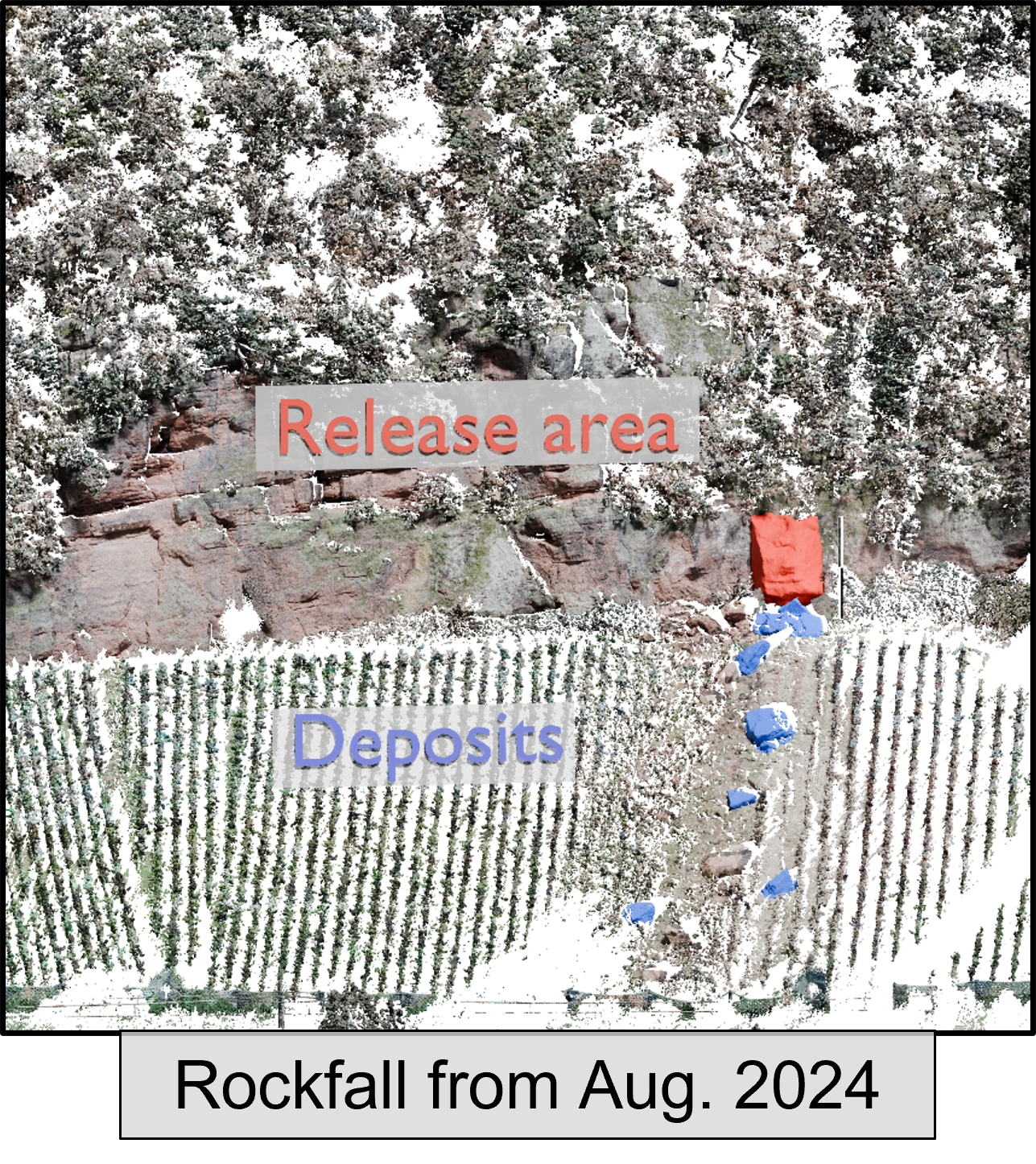
The figure shows the rock outcrop from the front. The red area marks the release area, where material was detached from the slope, and the blue areas mark the deposits. These are the surface changes that we want to detect in the point clouds.
Learning Objectives:
- Use VAPC occupancy differences as a coarse screening for appeared and disappeared geometry.
- Use bitemporal Mahalanobis distances to detect changed point distributions inside shared voxels.
- Build a candidate mask that keeps both occupancy-only changes and significant distribution changes.
- Map candidate voxels back to original point clouds for detailed analysis.
- Compare full-scene M3C2 with a hierarchical M3C2 run.
- Explain why the final change analysis can combine voxel features, M3C2 distances, spatial clusters, and domain interpretation.
Dataset
The test site is the same Trier rockfall-prone slope used in Activity 3.1. It is monitored hourly with a permanently installed RIEGL VZ-2000i terrestrial laser scanner. The two epochs used here were acquired one hour apart on August 26, 2024: one immediately before a rockfall and one immediately after it. In this notebook the target epoch is assumed to be registered already, so the focus shifts from alignment to efficient change detection.
Hierarchical change analysis
The first step is deliberately coarse: compare voxel occupancy and point distributions instead of individual point distances. This is useful in rockfall monitoring because vegetation and rock surfaces can both change between epochs, but their point distributions inside a voxel are often different.
Vegetation usually produces a scattered 3D point distribution. A rock wall is more plane-like. VAPC uses the point distribution inside each voxel, including covariance, to compare the two epochs. The Mahalanobis distance then measures change relative to this local distribution, not just as a Euclidean distance between two points.
An important aspect is that the voxel-based change detection is not the final deformation result. It is a fast candidate selection step.
The hierarchical idea is therefore:
- Use occupancy differences to keep voxels that are present in only one epoch.
- Use Mahalanobis screening for voxels occupied in both epochs.
- Run expensive point-based analysis only in the resulting candidate area.
- Use those candidate areas as input for later event classification.
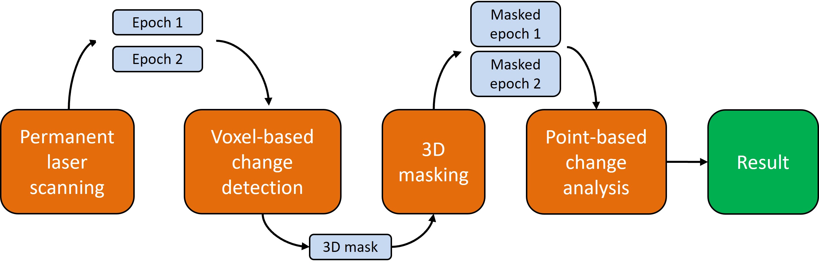
Hierarchical change analysis workflow for permanent laser scanning change analysis. Voxel-based detection first identifies candidate regions and creates a 3D mask. The masked epochs are then passed to point-based change analysis, reducing computation and supporting later change-event filtering and classification as used in AImon5.0.
Setup and Data Loading
First, we import the required libraries and disable verbose py4dgeo tracing so the notebook output stays focused on the analysis.
from pathlib import Path
import time
import py4dgeo
import numpy as np
import matplotlib.pyplot as plt
from matplotlib.lines import Line2D

py4dgeo.enable_trace(False)
py4dgeo.enable_timeit(False)
We use the same rockfall study area as in Activity 3.1. For this notebook the target epoch is assumed to be registered already, because the focus is event screening rather than co-registration. The file paths therefore point to the two registered epochs.
data_path = Path("../data/activity_3_1_and_3_3/point_clouds")

reference_path = data_path / "ScanPos001 - SINGLESCANS - 240826_000005_registered.laz"
target_path = data_path / "ScanPos001 - SINGLESCANS - 240826_010006_registered.laz"

reference_epoch = py4dgeo.read_from_las(reference_path)
target_epoch = py4dgeo.read_from_las(target_path)

print(f"Reference points: {reference_epoch.cloud.shape[0]:,}")
print(f"Target points:    {target_epoch.cloud.shape[0]:,}")
[2026-06-23 19:00:11][INFO] Reading point cloud from file 'D:\extract_4d\isprs_course\activity_3_1_and_3_3\point_clouds\ScanPos001 - SINGLESCANS - 240826_000005_registered.laz'
[2026-06-23 19:00:11][INFO] Reading point cloud from file 'D:\extract_4d\isprs_course\activity_3_1_and_3_3\point_clouds\ScanPos001 - SINGLESCANS - 240826_010006_registered.laz'
Reference points: 1,096,110
Target points:    1,147,552
Coarse occupancy comparison
This is where we stopped in Activity 2.4: we first ask which voxels are occupied only in epoch 1, only in epoch 2, or in both epochs. Occupancy-only changes are useful context and must remain part of the analysis. The following Mahalanobis step adds information only for voxels that are occupied in both epochs.
The voxel size controls how coarse this first screening is. A 4 m voxel is intentionally broad: it is not meant to outline the rockfall precisely, but to identify parts of the scene worth inspecting in more detail.
voxel_size_change_detection = 4.0

vapc_reference = py4dgeo.Vapc(reference_epoch, voxel_size=voxel_size_change_detection)
vapc_target = py4dgeo.Vapc(target_epoch, voxel_size=voxel_size_change_detection)

occupancy_change = vapc_reference.delta_vapc(vapc_target)
occupancy_type = occupancy_change.out["delta_vapc"]

only_reference = occupancy_type == 1
only_target = occupancy_type == 2
occupied_both = occupancy_type == 3

print(f"Voxel size for change detection: {voxel_size_change_detection} m")
print(f"Only epoch 1:     {only_reference.sum():,} voxels")
print(f"Only epoch 2:     {only_target.sum():,} voxels")
print(f"Occupied in both: {occupied_both.sum():,} voxels")
Voxel size for change detection: 4.0 m
Only epoch 1:     60 voxels
Only epoch 2:     65 voxels
Occupied in both: 3,292 voxels
Voxels that are occpuied in only one epoch do not provide a pair of distributions, but they are still changes candidated because geometry appeared or disappeared. We therefore keep occupancy-only voxels for the final candidate mask and apply the distribution test only to the shared voxels.
Before moving on, inspect the occupancy figure carefully. Blue voxels are places where points exist only in the reference epoch, red voxels exist only in the target epoch, and dark voxels are occupied in both epochs. In a rockfall scene, blue can indicate material loss, red can indicate newly visible or deposited material, and dark shared voxels are the places where distribution-based screening can add more evidence.
The first occupancy figure needs one color per voxel. The array occupancy_colors starts as transparent grey for all voxels, then the three occupancy classes overwrite that default color.
occupancy_colors = np.full(occupancy_type.shape, "#C7C7C73C", dtype=object)
occupancy_colors[only_reference] = "tab:blue"
occupancy_colors[only_target] = "tab:red"
occupancy_colors[occupied_both] = "#0A0A0A40"
The scatter plot uses the voxel-center coordinates stored in occupancy_change.epoch.cloud. Each square represents one voxel, not one original point.
fig = plt.figure(figsize=(9, 8))
ax = fig.add_subplot(projection="3d")
ax.scatter(
    occupancy_change.epoch.cloud[:, 0],
    occupancy_change.epoch.cloud[:, 1],
    occupancy_change.epoch.cloud[:, 2],
    c=occupancy_colors,
    s=20,
    marker="s",
)

ax.set_xlabel("X [m]")
ax.set_ylabel("Y [m]")
ax.set_zlabel("Z [m]")
ax.set_title("VAPC occupancy comparison")
ax.set_aspect("equal", "box")

legend_handles = [
    Line2D([0], [0], marker="s", color="w", label="only epoch 1", markerfacecolor="tab:blue", markersize=6),
    Line2D([0], [0], marker="s", color="w", label="only epoch 2", markerfacecolor="tab:red", markersize=6),
    Line2D([0], [0], marker="s", color="w", label="both epochs", markerfacecolor="#0A0A0A40", markersize=6),
]
ax.legend(handles=legend_handles, title="Voxel occupancy")
plt.show()

Distribution-based screening
For voxels occupied in both epochs, VAPC compares the local point distributions. This helps separate irregular vegetation motion from coherent rock-surface change: the same displacement can be insignificant in a scattered vegetation voxel, but significant on a compact rock surface.
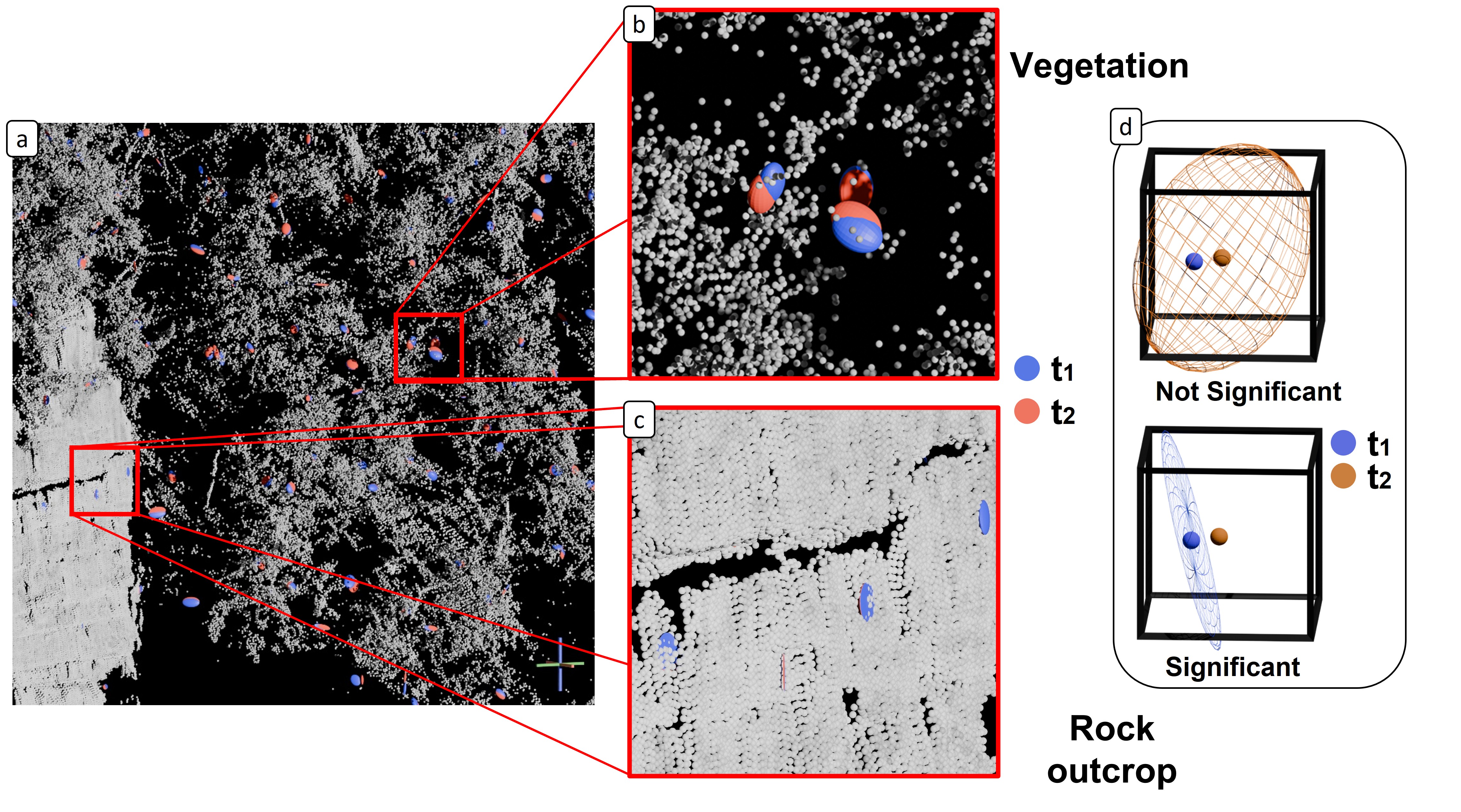
Distribution-based voxel screening in VAPC. Local point distributions are compared between two epochs using their mean positions and covariance structure. In vegetation, broad and irregular point distributions can make apparent motion statistically insignificant, whereas compact rock-surface distributions can make smaller, coherent displacements significant.
This screening uses parameters such as voxel size, minimum point count per voxel, and significance level. We keep these settings fixed here rather than tuning them in the notebook. Tabernig et al. (2025) discuss how these parameters influence detection and how suitable values can be selected.
Runtime is measured because the hierarchical workflow should be evaluated by both detection quality and computational cost.
mahalanobis_start = time.perf_counter()

mahalanobis_change = vapc_reference.compute_bitemporal_mahalanobis(
    vapc_target,
    min_points=30,
)

mahalanobis_elapsed = time.perf_counter() - mahalanobis_start
The Mahalanobis result stores several arrays. Here we convert them into named masks so the candidate logic is explicit: occupancy-only voxels are kept, and shared voxels are kept only when their distribution change is significant.
change_type = mahalanobis_change.out["change_type"]
mahalanobis_distance = mahalanobis_change.out["mahalanobis"]
significant = mahalanobis_change.out["significance"].astype(bool)

only_reference_change = change_type == 1
only_target_change = change_type == 2
shared_voxels = change_type == 3
distribution_candidate_voxels = shared_voxels & significant # Voxels occupied in both epochs AND significant intra-voxel change
candidate_voxels = only_reference_change | only_target_change | distribution_candidate_voxels # Occupied only in Epoch1 OR only in Epoch 2 OR (Occupied in both AND significant intra-voxel change)

print(f"Mahalanobis screening time:              {mahalanobis_elapsed:.1f} s")
print(f"Only epoch 1 voxels:                     {only_reference_change.sum():,}")
print(f"Only epoch 2 voxels:                     {only_target_change.sum():,}")
print(f"Shared voxels:                           {shared_voxels.sum():,}")
print(f"Significant shared distribution changes: {distribution_candidate_voxels.sum():,}")
print(f"Total candidate voxels:                  {candidate_voxels.sum():,}")
Mahalanobis screening time:              0.3 s
Only epoch 1 voxels:                     60
Only epoch 2 voxels:                     65
Shared voxels:                           3,292
Significant shared distribution changes: 1,437
Total candidate voxels:                  1,562
The next plot separates the candidate voxels by source. This keeps occupancy-only candidates visible while highlighting shared voxels where the intra-voxel distribution changed significantly. The code is split into two parts: first we prepare the voxel groups, then we plot them. This makes it easier to connect each color in the figure to the boolean masks created above.
# First we prepare the voxel groups
context_voxels = ~candidate_voxels
voxels_context = mahalanobis_change.epoch.cloud[context_voxels]
voxels_only_reference = mahalanobis_change.epoch.cloud[only_reference_change]
voxels_only_target = mahalanobis_change.epoch.cloud[only_target_change]
voxels_distribution_change = mahalanobis_change.epoch.cloud[distribution_candidate_voxels]
In the candidate figure, grey voxels are context only. Blue and red are occupancy-only candidates, while orange marks shared voxels whose point distribution changed significantly. The plot is therefore a screening map, not yet a final rockfall-event map.
fig = plt.figure(figsize=(9, 8))
ax = fig.add_subplot(projection="3d")

ax.scatter(
    voxels_context[:, 0],
    voxels_context[:, 1],
    voxels_context[:, 2],
    c="0.8",
    s=1,
    marker="s",
)
ax.scatter(
    voxels_only_reference[:, 0],
    voxels_only_reference[:, 1],
    voxels_only_reference[:, 2],
    c="tab:blue",
    s=15,
    marker="s",
)
ax.scatter(
    voxels_only_target[:, 0],
    voxels_only_target[:, 1],
    voxels_only_target[:, 2],
    c="tab:red",
    s=15,
    marker="s",
)
ax.scatter(
    voxels_distribution_change[:, 0],
    voxels_distribution_change[:, 1],
    voxels_distribution_change[:, 2],
    c="tab:orange",
    s=15,
    marker="s",
)

ax.set_xlabel("X [m]")
ax.set_ylabel("Y [m]")
ax.set_zlabel("Z [m]")
ax.set_title("Hierarchical candidate voxels")
ax.set_aspect("equal", "box")

legend_handles = [
    Line2D([0], [0], marker="s", color="w", label="no candidate", markerfacecolor="0.8", markersize=6),
    Line2D([0], [0], marker="s", color="w", label="only occupied in epoch 1", markerfacecolor="tab:blue", markersize=6),
    Line2D([0], [0], marker="s", color="w", label="only occupied in epoch 2", markerfacecolor="tab:red", markersize=6),
    Line2D([0], [0], marker="s", color="w", label="significant intra-voxel change", markerfacecolor="tab:orange", markersize=6),
]
ax.legend(handles=legend_handles, title="Candidate source", loc="upper left", bbox_to_anchor=(1.02, 1.0))
plt.tight_layout()
plt.show()

Points within candidate voxels
The candidate voxels are a compact area for detailed follow-up change analysis. We map them back to both original high-resolution point clouds, because occupancy-only changes can occur in either epoch. This is the step where the coarse voxel screen becomes a point-cloud subset again.
For the reference-based M3C2 comparison below, core points can only be selected from candidate voxels that contain reference points. Therefore, the reference-backed M3C2 candidate set includes voxels occupied only in epoch 1 and significant shared voxels. Voxels occupied only in epoch 2 remain part of the event candidate map and can be handled by a reverse M3C2 run or by later voxel/cluster classification.
candidate_vapc = mahalanobis_change.filter(candidate_voxels, overwrite=False)
candidate_reference, candidate_reference_point_mask = vapc_reference.select_by_mask(candidate_vapc)
candidate_target, candidate_target_point_mask = vapc_target.select_by_mask(candidate_vapc)

reference_points_within_candidate_voxels = candidate_reference.epoch.cloud
target_points_within_candidate_voxels = candidate_target.epoch.cloud
The next mask is narrower. It keeps only candidate voxels that can provide reference core points for this forward M3C2 run. This is why only_target_change is not included in m3c2_candidate_voxels.
m3c2_candidate_voxels = only_reference_change | distribution_candidate_voxels
m3c2_candidate_vapc = mahalanobis_change.filter(m3c2_candidate_voxels, overwrite=False)
m3c2_candidate_reference, m3c2_candidate_point_mask = vapc_reference.select_by_mask(m3c2_candidate_vapc)
points_for_hierarchical_m3c2 = m3c2_candidate_reference.epoch.cloud

print(f"Total candidate voxels:                    {candidate_voxels.sum():,}")
print(f"Reference points in candidate voxels:      {reference_points_within_candidate_voxels.shape[0]:,}")
print(f"Target points in candidate voxels:         {target_points_within_candidate_voxels.shape[0]:,}")
print(f"Reference-backed M3C2 candidate voxels:    {m3c2_candidate_voxels.sum():,}")
print(f"Reference-backed points for M3C2:          {points_for_hierarchical_m3c2.shape[0]:,}")
print(f"Reference M3C2 reduction vs full scene:    {reference_epoch.cloud.shape[0] / max(points_for_hierarchical_m3c2.shape[0], 1):.1f}x"
)
Total candidate voxels:                    1,562
Reference points in candidate voxels:      139,977
Target points in candidate voxels:         163,229
Reference-backed M3C2 candidate voxels:    1,497
Reference-backed points for M3C2:          139,977
Reference M3C2 reduction vs full scene:    7.8x
M3C2 with and without hierarchical screening
Now we run M3C2 twice with the same settings. The left plot uses spatially subsampled core points from the whole reference epoch. The right plot uses only reference-backed points inside hierarchical candidate voxels. Both runs use the same core point spacing and M3C2 radius so that the comparison focuses on the effect of hierarchical screening.
The M3C2 cells can compute for a little while. That is expected.: the full-scene run searches neighborhoods around many more core points, whereas the hierarchical run should be faster because the voxel screen has already removed much of the scene.
# Define shared M3C2 parameters
m3c2_corepoint_voxel_size = 0.5
m3c2_radius = 2.0
m3c2_parameters = {
    "cyl_radius": m3c2_radius,
    "normal_radii": [m3c2_radius],
}


# Extract core points from full scene
full_scene_vapc = py4dgeo.Vapc(reference_epoch, voxel_size=m3c2_corepoint_voxel_size)
full_scene_corepoints = full_scene_vapc.reduce_to_feature("closest_to_voxel_centers").epoch.cloud

# Extract core points from reduced candidate area
candidate_point_epoch = py4dgeo.Epoch(points_for_hierarchical_m3c2.copy())
candidate_corepoint_vapc = py4dgeo.Vapc(candidate_point_epoch, voxel_size=m3c2_corepoint_voxel_size)
candidate_corepoints = candidate_corepoint_vapc.reduce_to_feature("closest_to_voxel_centers").epoch.cloud
C:\Users\nc298\repos\small_gicp\small_gicp\src\py4dgeo\src\py4dgeo\vapc.py:175: UserWarning: Numba is not installed. Vapc uses slower NumPy fallbacks.
  _warn_numba_missing_once()
The helper function below keeps the two M3C2 runs comparable: it prints the number of core points, measures runtime, and returns the same result structure for both runs.
def run_timed_m3c2(label, corepoints):
    print(f"Running M3C2 for {label}: {corepoints.shape[0]:,} core points")
    start = time.perf_counter()
    algorithm = py4dgeo.M3C2(
        epochs=(reference_epoch, target_epoch),
        corepoints=corepoints,
        **m3c2_parameters,
    )
    distances, uncertainties = algorithm.run()
    elapsed = time.perf_counter() - start
    print(f"Finished {label} in {elapsed:.1f} s")
    return {
        "label": label,
        "corepoints": corepoints,
        "distances": distances,
        "uncertainties": uncertainties,
        "elapsed": elapsed,
    }
We now call the helper twice. The first call is the baseline full-scene analysis; the second call is the hierarchical analysis.
m3c2_comparison_results = [
    run_timed_m3c2("without hierarchical screening", full_scene_corepoints),
    run_timed_m3c2("with hierarchical screening", candidate_corepoints),
]
Running M3C2 for without hierarchical screening: 188,976 core points
Finished without hierarchical screening in 3.4 s
Running M3C2 for with hierarchical screening: 31,284 core points
Finished with hierarchical screening in 0.3 s
Finally, we visualize both M3C2 runs with the same color scale. Red indicates negative M3C2 distances and blue indicates positive distances. The important comparison is not only the color pattern, but also the number of core points and runtime printed in each panel title. If the right panel keeps the relevant rockfall signal while using far fewer core points, the hierarchical screen has done its job.
valid_distances = np.concatenate([
    result["distances"][np.isfinite(result["distances"])]
    for result in m3c2_comparison_results
])
if valid_distances.size == 0:
    raise ValueError("No finite M3C2 distances available for plotting.")

vmax = 0.5
The plotting cell uses the same loop for both panels.
fig, axes = plt.subplots(
    1,
    2,
    figsize=(14, 6),
    subplot_kw={"projection": "3d"},
    constrained_layout=True,
)

for ax, result in zip(axes, m3c2_comparison_results):
    corepoints = result["corepoints"]
    distances = result["distances"]
    finite = np.isfinite(distances)
    plot_step = max(1, finite.sum() // 100_000)

    sc = ax.scatter(
        corepoints[finite, 0][::plot_step],
        corepoints[finite, 1][::plot_step],
        corepoints[finite, 2][::plot_step],
        c=distances[finite][::plot_step],
        cmap="coolwarm_r",
        vmin=-vmax,
        vmax=vmax,
        s=0.5,
    )
    ax.set_title(
        f"{result['label']}\n"
        f"{corepoints.shape[0]:,} core points, M3C2 {result['elapsed']:.1f} s"
    )
    ax.set_xlabel("X [m]")
    ax.set_ylabel("Y [m]")
    ax.set_zlabel("Z [m]")
    ax.set_aspect("equal", "box")

cbar = fig.colorbar(sc, ax=axes, shrink=0.65, pad=0.04)
cbar.set_label("M3C2 distance [m]")

hierarchical_total_elapsed = mahalanobis_elapsed + m3c2_comparison_results[1]["elapsed"]
caption = (
    f"Screening time: {mahalanobis_elapsed:.1f} s. "
    f"Hierarchical total: screening + candidate M3C2 = {hierarchical_total_elapsed:.1f} s. "
    f"\nCore-point spacing: {m3c2_corepoint_voxel_size:g} m; M3C2 radius: {m3c2_radius:g} m."
)
fig.text(0.5, -0.04, caption, ha="center", fontsize=15)
plt.show()

The above figure shows how the hierarchical change analysis approach drastically reduces the area of interest, while retaining the actual rockfall event in the data. This illustrates the fundamental trade-off situation we are facing. On the one hand, we want to reduce the data as much as possible; on the other hand, we want to maintain all parts of the data that contain areas with actual surface changes. The tricky part is finding parameters that satisfy both requirements. How these parameters can be determined is described by Tabernig et al. (2025).
References
- Tabernig, R., Albert, W., Weiser, H., & Höfle, B. (2025). A hierarchical approach for near real-time 3D surface change analysis of permanent laser scanning point clouds. In: 6th Joint International Symposium on Deformation Monitoring (JISDM). doi: 10.5445/IR/1000180377.
- Albert, W., Tabernig, R., & Höfle, B. (2025). AImon5.0 (Version 1.0.0). https://github.com/3dgeo-heidelberg/AImon.